Folders
Files
DESCRIPTION
index.html
next_motif.gif
PACKAGES
previous_motif.gif
R-logo.gif
Simple_0.6.tar.gz
Simple_0.6.zip
simpleR.R
stat.html
stat001.gif
stat001.html
stat002.gif
stat002.html
stat003.gif
stat003.html
stat004.gif
stat004.html
stat005.gif
stat005.html
stat006.gif
stat006.html
stat007.gif
stat007.html
stat008.gif
stat008.html
stat009.gif
stat009.html
stat010.gif
stat010.html
stat011.gif
stat011.html
stat012.gif
stat012.html
stat013.gif
stat013.html
stat014.gif
stat014.html
stat015.gif
stat015.html
stat016.gif
stat016.html
stat017.gif
stat017.html
stat018.gif
stat018.html
stat019.gif
stat019.html
stat020.gif
stat020.html
stat021.gif
stat021.html
stat022.gif
stat022.html
stat023.gif
stat023.html
stat024.gif
stat024.html
stat025.gif
stat025.html
stat026.gif
stat026.html
stat027.gif
stat028.gif
stat029.gif
stat030.gif
stat031.gif
stat032.gif
stat033.gif
stat034.gif
stat035.gif
stat036.gif
stat037.gif
stat038.gif
stat039.gif
stat040.gif
stat041.gif
stat042.gif
stat043.gif
stat044.gif
stat045.gif
stat046.gif
stat047.gif
stat048.gif
stat049.gif
stat050.gif
stat051.gif
stat052.gif
stat053.gif
stat054.gif
stat055.gif
stat056.gif
stat057.gif
stat058.gif
stat059.gif


9 Confidence Interval Estimation
In statistics one often would like to estimate unknown parameters for a known distribution. For example, you may think that your parent population is normal, but the mean is unknown, or both the mean and standard deviation are unknown. From a data set you can't hope to know the exact values of the parameters, but the data should give you a good idea what they are. For the mean, we expect that the sample mean or average of our data will be a good choice for the population mean, and intuitively, we understand that the more data we have the better this should be. How do we quantify this?Statistical theory is based on knowing the sampling distribution of some statistic such as the mean. This allows us to make probability statements about the value of the parameters. Such as we are 95 percent certain the parameter is in some range of values.
In this section, we describe the R functions prop.test, t.test, and wilcox.test used to facilitate the calculations.
9.1 Population proportion theory
The most widely seen use of confidence intervals is the estimation of population proportion through surveys or polls. For example, suppose it is reported that 100 people were surveyed and 42 of them liked brand X. How do you see this in the media?Depending on the sophistication of the reporter, you might see the claim that 42% of the population reports they like brand X. Or, you might see a statement like ``the survey indicates that 42% of people like brand X, this has a margin of error of 9 percentage points.'' Or, if you find an extra careful reporter you will see a summary such as ``the survey indicates that 42% of people like brand X, this has a margin of error of 9 percentage points. This is a 95% confidence level.''
Why all the different answers? Well, the idea that we can infer anything about the population based on a survey of just 100 people is founded on probability theory. If the sample is a random sample then we know the sampling distribution of p^ the sample proportion. It is approximately normal.
Let's fix the notation. Suppose we let p be the true population proportion, which is of course
| p = |
|
|
= |
|
. |
We could say more. If the sampled answers are recorded as Xi where Xi = 1 if it was ``yes'' and Xi = 0 if ``no'', then our sample is {X1,X2,...,Xn} where n is the size of the sample and we get
|
= |
|
. |
Now if we satisfy the assumptions that each Xi is i.i.d. then p^ has a known distribution, and if n is large enough we can say the following is approximately normal with mean 0 and variance 1:
| z = |
|
= |
|
If we know this, then we can say how close z is to zero by specifying a confidence. For example, from the known properties of the normal, we know that
- z is in (-1,1) with probability approximately 0.68
- z is in (-2,2) with probability approximately 0.95
- z is in (-3,3) with probability approximately 0.998
| ( | p(1-p)/n | ) |
|
| P(-1 < |
|
< 1) = .68, P(-2 < |
|
< 2) = .95, P(-3 < |
|
< 3) = .998, |
Or in particular, on average 95% of the time the interval (p^ - 2SE,p^+2SE) contains the true value of p. In the words of a reporter this would be a 95% confidence level, an ``answer'' of p^=.42 with a margin of error of 9 percentage points (2*SE in percents).
More generally, we can find the values for any confidence level. This is usually denoted in reverse by calling it a (1-a)100% confidence level. Where for any a in (0,1) we can find a z* with
P(-z* < z < z*) = 1-a
Often such a z* is called z1-a/2 from how it is
found. For R this can be found with the qnorm function
> alpha = c(0.2,0.1,0.05,0.001)
> zstar = qnorm(1 - alpha/2)
> zstar
[1] 1.281552 1.644854 1.959964 3.290527
Notice the value z* = 1.96 corresponds to a=.05 or a 95% confidence interval. The reverse is done with the pnorm function:
> 2*(1-pnorm(zstar))
[1] 0.200 0.100 0.050 0.001
In general then, a (1-a)100% confidence interval is then given by
|
± z* SE |
Does this agree with intuition? We should expect that as n gets bigger we have more confidence. This is so because as n gets bigger, the SE gets smaller as there is a
| ( | n | ) |
|
Some Extra Insight: Confidence interval isn't always right
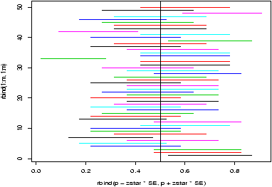
The fact that not all confidence intervals contain the true value of the parameter is often illustrated by plotting a number of random confidence intervals at once and observing. This is done in figure 43.
The fact that not all confidence intervals contain the true value of the parameter is often illustrated by plotting a number of random confidence intervals at once and observing. This is done in figure 43.
This was quite simply generated using the command matplot
> m = 50; n=20; p = .5;         # toss 20 coins 50 times
> phat = rbinom(m,n,p)/n        # divide by n for proportions
> SE = sqrt(phat*(1-phat)/n)    # compute SE
> alpha = 0.10;zstar = qnorm(1-alpha/2)
> matplot(rbind(phat - zstar*SE, phat + zstar*SE),
+ rbind(1:m,1:m),type="l",lty=1)
> abline(v=p)                  # draw line for p=0.5
Many other tests follow a similar pattern:
- One finds a ``good'' statistic that involves the unknown parameter (a pivotal quantity).
- One uses the known distribution of the statistic to make a probabilistic statement.
- One unwraps things to form a confidence interval. This is often of the form the statistic plus or minus a multiple of the standard error although this depends on the ``good'' statistic.
9.2 Proportion test
Let's use R to find the above confidence level10. The main R command for this is prop.test (proportion test). To use it to find the 95% confidence interval we do
> prop.test(42,100)

     1-sample proportions test with continuity correction

data:  42 out of 100, null probability 0.5
X-squared = 2.25, df = 1, p-value = 0.1336
alternative hypothesis: true p is not equal to 0.5
95 percent confidence interval:
 0.3233236 0.5228954
sample estimates:
   p
0.42
Notice, in particular, we get the 95% confidence interval
(0.32,0.52) by default. If we want a 90% confidence interval we need to ask for it:
>  prop.test(42,100,conf.level=0.90)

     1-sample proportions test with continuity correction

data:  42 out of 100, null probability 0.5
X-squared = 2.25, df = 1, p-value = 0.1336
alternative hypothesis: true p is not equal to 0.5
90 percent confidence interval:
 0.3372368 0.5072341
sample estimates:
   p
0.42
Which gives the interval (0.33,0.50). Notice this is smaller as we
are now less confident.
Some Extra Insight: prop.test is more accurate
The results of prop.test will differ slightly than the results found as described previously. The prop.test function actually starts from
and then solves for an interval for p. This is more complicated
algebraically, but more correct, as the central limit theorem
approximation for the binomial is better for this expression.
The results of prop.test will differ slightly than the results found as described previously. The prop.test function actually starts from
| | |
|
| < z* |
9.3 The z-test
As above, we can test for the mean in a similar way, provided the statistic
|
- s is known, and the Xi's are normally distributed.
- s is known, and n is large enough to apply the CLT.
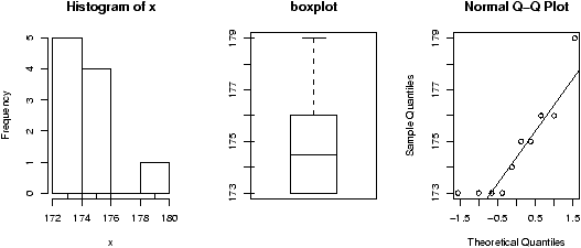
175 176 173 175 174 173 173 176 173 179
Suppose that s=1.5 and the error in weighing is normally distributed. (That is Xi = µ + ei where ei is normal with mean 0 and standard deviation 1.5). Rather than use a built-in test, we illustrate how we can create our own:
## define a function
> simple.z.test = function(x,sigma,conf.level=0.95) {
+ n = length(x);xbar=mean(x)
+ alpha = 1 - conf.level
+ zstar = qnorm(1-alpha/2)
+ SE = sigma/sqrt(n)
+ xbar + c(-zstar*SE,zstar*SE)
+ }
## now try it
> simple.z.test(x,1.5)
[1] 173.7703 175.6297
Notice we get the 95% confidence interval of (173.7703, 175.6297)
9.4 The t-test
More realistically, you may not know the standard deviation. To work around this we use the t-statistic, which is given by| t = |
|
- The Xi are normal and n is small then this has the t-distribution with n-1 degrees of freedom.
- If n is large then the CLT applies and it is approximately normal. (In most cases.)
Lets suppose in our weight example, we don't assume the standard deviation is 1.5, but rather let the data decide it for us. We then would use the t-test provided the data is normal (Or approximately normal.). To quickly investigate this assumption we look at the qqnorm plot and others
Things pass for normal (although they look a bit truncated on the left end) so we apply the t-test. To compare, we will do a 95% confidence interval (the default)
> t.test(x)

     One Sample t-test

data:  x
t = 283.8161, df = 9, p-value = < 2.2e-16
alternative hypothesis: true mean is not equal to 0
95 percent confidence interval:
 173.3076 176.0924
sample estimates:
mean of x
    174.7
Notice we get a different confidence interval.
Some Extra Insight: Comparing p-values from t and z
One may be tempted to think that the confidence interval based on the t statistic would always be larger than that based on the z statistic as always t* > z* . However, the standard error SE for the t also depends on s which is variable and can sometimes be small enough to offset the difference.
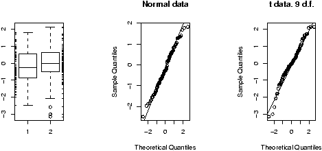
To see why t* is always larger than z*, we can compare side-by-side boxplots of two random sets of data with these distributions.
> x=rnorm(100);y=rt(100,9)
> boxplot(x,y)
> qqnorm(x);qqline(x)
> qqnorm(y);qqline(y)
which gives (notice the symmetry of both, but the larger variance of the t distribution).
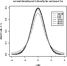
And for completeness, this creates a graph with several theoretical densities.
> xvals=seq(-4,4,.01)
> plot(xvals,dnorm(xvals),type="l")
> for(i in c(2,5,10,20,50)) points(xvals,dt(xvals,df=i),type="l",lty=i)
9.5 Confidence interval for the median
Confidence intervals for the median are important too. They are different mathematically than the ones above, but in R these differences aren't noticed. The R function wilcox.test performs a non-parametric test for the median.Suppose the following data is pay of CEO's in America in 2001 dollars11, then the following creates a test for the median
> x = c(110, 12, 2.5, 98, 1017, 540, 54, 4.3, 150, 432)
> wilcox.test(x,conf.int=TRUE)

     Wilcoxon signed rank test

data:  x
V = 55, p-value = 0.001953
alternative hypothesis: true mu is not equal to 0
95 percent confidence interval:
  33.0 514.5
Notice a few things:
- Unlike prop.test and t.test, we needed to specify that we wanted a confidence interval computed.
- For this data, the confidence interval is enormous as the size of the sample is small and the range is huge.
- We couldn't have used a t-test as the data isn't even close to normal.
9.6 Problems
- 9.1
- Create 15 random numbers that are normally distributed with mean 10 and s.d. 5. Find a 1-sample z-test at the 95% level. Did it get it right?
- 9.2
- Do the above 100 times. Compute what percentage is in a 95%
confidence interval. Hint: The following might prove useful
> f=function () mean(rnorm(15,mean=10,sd=5))
> SE = 5/sqrt(15)
> xbar = simple.sim(100,f)
> alpha = 0.1;zstar = qnorm(1-alpha/2);sum(abs(xbar-10) < zstar*SE)
[1] 87
> alpha = 0.05;zstar = qnorm(1-alpha/2);sum(abs(xbar-10) < zstar*SE)
[1] 92
> alpha = 0.01;zstar = qnorm(1-alpha/2);sum(abs(xbar-10) < zstar*SE)
[1] 98
- 9.3
- The t-test is just as easy to do. Do a t-test on the same data. Is it correct now? Comment on the relationship between the confidence intervals.
- 9.4
- Find an 80% and 95% confidence interval for the median for the exec.pay dataset.
- 9.5
- For the Simple data set rat do a t-test for mean if the data suggests it is appropriate. If not, say why not. (This records survival times for rats.)
- 9.6
- Repeat the previous for the Simple data set puerto (weekly incomes of Puerto Ricans in Miami.).
- 9.7
- The median may be the appropriate measure of center. If so, you might want to have a confidence interval for it too. Find a 90% confidence interval for the median for the Simple data set malpract (on the size of malpractice awards). Comment why this distribution doesn't lend itself to the z-test or t-test.
- 9.8
- The t-statistic has the t-distribution if the Xi's are
normally distributed. What if they are not? Investigate the
distribution of the t-statistic if the Xi's have different
distributions. Try short-tailed ones (uniform), long-tailed ones
(t-distributed to begin with), Uniform (exponential or log-normal).
(For example, If the Xi are nearly normal, but there is a chance of some errors introducing outliers. This can be modeled withXi = z(µ + s Z) + (1-z)Ywhere z is 1 with high probability and 0 otherwise and Y is of a different distribution. For concreteness, suppose µ=0, s=1 and Y is normal with mean 0, but standard deviation 10 and P(z=1) = .9. Here is some R code to simulate and investigate. (Please note, the simulations for the suggested distributions should be much simpler.)> f = function(n=10,p=0.95) { + y = rnorm(n,mean=0,sd=1+9*rbinom(n,1,1-p)) + t = (mean(y) - 0) / (sqrt(var(y))/sqrt(n)) + } > sample = simple.sim(100,f) > qqplot(sample,rt(100,df=9),main="sample vs. t");qqline(sample) > qqnorm(sample,main="sample vs. normal");qqline(sample) > hist(sample)The resulting graphs are shown. First, the graph shows the sample against the t-quantiles. A bad, fit. The normal plot is better but we still see a skew in the histogram due to a single large outlier.)
Copyright © John Verzani, 2001-2. All rights reserved.


