---

20  Using Functions

In R the use of functions allows the user to easily extend and simplify the R session. In fact, most of R, as distributed, is a series of R functions. In this appendix, we learn a little bit about creating your own functions.

20.1  The basic template

The basic template for a function is

function_name <- function (function_arguments) {
  function_body
  function_return_value
}
  

Each of these is important. Let's cover them in the order they appear

function_name

The function name, can be just about anything -- even functions or variables previously defined so be careful. Once you have given the name, you can use it just like any other function -- with parentheses. For example to define a standard deviation function using the var function we can do

> std <- function (x) sqrt(var(x))    
  

This has the name std. It is used thusly

> data <- c(1,3,2,4,1,4,6)    
> std(data)
[1] 1.825742
  

If you call it without parentheses you will get the function definition itself

> std
function (x) sqrt(var(x))    
  

The keyword function

Notice in the definition there is always the keyword function informing R that the new object is of the function class. Don't forget it.

The function_arguments

The arguments to a function range from straightforward to difficult. Here are some examples

No arguments

Sometimes, you use a function just as a convenience and it always does the same thing, so input is not important. An example might be the ubiquitous ``hello world'' example from just about any computer science book

> hello.world <- function() print("hello world")      
> hello.world()
[1] "hello world"    
    

An argument

If you want to personalize this, you can use an argument for the name. Here is an example

> hello.someone <- function(name) print(paste("hello ",name))
> hello.someone("fred")
[1] "hello  fred"
    

First, we needed to paste the words together before printing. Once we get that right, the function does the same thing only personalized.

A default argument

What happens if you try this without an argument? Let's see

> hello.someone()
Error in paste("hello ", name) : Argument "name" is missing, with no default
    

Hmm, an error, we should have a sensible default. R provides an easy way for the function writer to provide defaults when you define the function. Here is an example

> hello.someone <- function(name="world") print(paste("hello ",name)) 
> hello.someone()
[1] "hello  world"
    

Notice argument = default_value. After the name of the variable, we put an equals sign and the default value. This is not assignment, which is done with the <-. One thing to be aware of is the default value can depend on the data as R practices lazy evaluation. For example

> bootstrap = function(data,sample.size = length(data) {....      
    

Will define a function where the sample size by default is the size of the data set.

Now, if we are using a single argument, the above should get you the general idea. There is more to learn though if you are passing multiple parameters through.

Consider, the definition of a function for simulating the t statistic from a sample of normals with mean 10 and standard deviation 5.

> sim.t <- function(n) {
+ mu <- 10;sigma<-5;
+ X <- rnorm(n,mu,sigma)
+ (mean(X) - mu)/(sd(X)/n)
+ }
> sim.t(4)
[1] -1.574408   
  

This is fine, but what if you want to make the mean and standard deviation variable. We can keep the 10 and 5 as defaults and have

> sim.t <- function(n,mu=10,sigma=5) {
+ X <- rnorm(n,mu,sigma)
+ (mean(X) - mu)/(sd(X)/n)
+ }

Now, note how we can call this function

> sim.t(4)                      # using defaults
[1] -0.4642314
> sim.t(4,3,10)                 # n=4,mu=3, sigma=10
[1] 3.921082
> sim.t(4,5)                    # n=4,mu=5,sigma the default 5
[1] 3.135898
> sim.t(4,sigma=100)            # n-4,mu the default 10, sigma=100
[1] -9.960678
> sim.t(4,sigma=100,mu=1)       # named arguments don't need order
[1] 4.817636
  

We see, that we can use the defaults or not depending on how we call the function. Notice we can mix positional arguments and named arguments. The positional arguments need to match up with the order that is defined in the function. In particular, the call sim.t(4,3,10) matches 4 with n, 3 with mu and 10 with sigma, and sim.t(4,5) matches 4 with n, 5 with mu and since nothing is in the third position, it uses the default for sigma. Using named arguments, such as sim.t(4,sigma=100,mu=1) allows you to switch the order and avoid specifying all the values. For arguments with lots of variables this is very convenient.

There is one more possibility that is useful, the ... variable . This means, take these values and pass them on to an internal function. This is useful for graphics. For example to plot a function, can be tedious. You define the values for x, apply the values to create y and then plot the points using the line type. (Actually, the curve function does this for you). Here is a function that will do this

> plot.f <- function(f,a,b,...) {    
+ xvals<-seq(a,b,length=100)
+ plot(xvals,f(xvals),type="l",...)
+ }
  

Then plot.f(sin,0,2*pi) will plot the sine curve from 0 to 2p and plot.f(sin,0,2*pi,lty=4) will do the same, only with a different way of drawing the line.

The function_body and function_return_value

The body of the function and its return value do the work of the function. The value that gets returned is the last thing evaluated. So if only one thing is found, it is easy to write a function. For example, here is a simple way of defining an average

> our.average <- function (x) sum(x)/length(x)    
> our.average(c(1,2,3))         # average of 1,2,3 is 2
[1] 2
  

Of course the function mean does this for you -- and more (trimming, removal of NA etc.).

If your function is more complicated, then the function's body and return value are enclosed in braces: {}.

In the body, the function may use variables. usually these are arguments to the function. What if they are not though? Then R goes hunting to see what it finds. Here is a simple example. Where and how R goes hunting is the topic of scope which is covered more thoroughly in some of the other documents listed in the ``Sources of help, documentation'' appendix.

> x<-c(1,2,3)                   # defined outside the function
> our.average()
[1] 2
> rm(x)
> our.average()
Error in sum(x) : Object "x" not found
  

20.2  For loops

A for loop allows you to loop over values in a vector or list of numbers. It is a powerful programming feature. Although, often in R one writes functions that avoid for loops in favor of those using a vector approach, a for loop can be a useful thing. When learning to write functions, they can make the thought process much easier.

Here are some simple examples. First we add up the numbers in the vector x (better done with sum)

> silly.sum <- function (x) {
+ ret <- 0;
+ for (i in 1:length(x)) ret <- ret + x[i]
+ ret
+ }
> silly.sum(c(1,2,3,4))
[1] 10
  

Notice the line for (i in 1:length(x)) ret <- ret + x[i]. This has the basic structure

for (variable in vector) {
   expression(s)
}    
  

where in this example variable is i, the vector is 1,2,...length(x) (to get at the indices of x) and the expression is the single command ret <- ret + x[i] which adds the next value of x to the previous sum. If there is more than one expression, then we can use braces as with the definition of a function.

(R's for loops are better used in this example to loop over the values in the vector x and not the indices as in

> for ( i in x) ret <- ret + i    
  

)

Here is an example that is more useful. Suppose you want to plot something for various values of a parameter. In particular, lets graph the t distribution for 2,5,10 and 25 degrees of freedom. (Use par(mfrow=c(2,2)) to get this all on one graph)

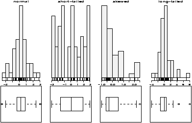
for (i in c(2,5,10,25))  hist(rt(100,df=i),breaks=10)
  

20.3  Conditional expressions

Conditional expressions allow you to do different things based on the value of a variable. For example, a naive definition of the absolute value function could look like this

> abs.x <- function(x) {
+ if (x<0) {x <- -x}
+ x
+ }
> abs.x(3)
[1] 3
> abs.x(-3)
[1] 3
> abs.x(c(-3,3))                # hey this is broken for vectors!
[1]  3 -3
  

The last line clearly shows, we could do much better than this (try x[x<0]<- -x[x<0] or the built in function abs). However, the example should be clear. If x is less than 0, then we set it equal to -x just as an absolute value function should.

The basic template is

if (condition) expression    
  

or

if (condition) {
  expression(s) if true
} else {
  expression(s) to do otherwise
}

There is much, much more to function writing in R. The topic is covered nicely in some of the materials mentioned in the appendix ``Sources of help, documentation''.

---