Files
der-1.gif
der-2.gif
dt-1.gif
dt-2.gif
dt-20.gif
dt-3.gif
dt-4.gif
fig-1.gif
index.html
lim-1.gif
MatlabPlotting.mp4
MatlabPlottingR2018a.mp4
newtons-method.gif
next_motif.gif
plt-8.gif
plts-1.gif
plts-2.gif
plts-3.gif
plts-4.gif
plts-5.gif
plts-6.gif
plts-7.gif
plts-7a.gif
previous_motif.gif
projectile-motion.mp4
projectile-motionR2018a.mp4
salary.mp4
salaryR2019a.mp4
shrt-1.gif
sin365.mp4
sin365R2018a.mp4
test.gif
tutorial-pieces.html
tutorial.html
tutorial001.gif
tutorial001.html
tutorial002.gif
tutorial002.html
tutorial003.gif
tutorial003.html
tutorial004.gif
tutorial004.html
tutorial005.gif
tutorial005.html
tutorial006.gif
tutorial006.html
tutorial007.gif
tutorial007.html
tutorial008.gif
tutorial008.html
tutorial009.gif
tutorial009.html
tutorial010.gif
tutorial010.html
tutorial011.gif
tutorial011.html
tutorial012.gif
tutorial012.html
tutorial013.gif
tutorial013.html
tutorial014.gif
tutorial014.html
tutorial015.gif
tutorial015.html
tutorial016.gif
tutorial017.gif
tutorial018.gif
tutorial019.gif
tutorial020.gif
tutorial021.gif
tutorial022.gif
zer-1.gif
zer-1a.gif
zer-2.gif
zer-3.gif


9 Derivatives
9.1 Difference quotients
Concept: Definition of a derivative
Let f(x) be a function defined in a neighborhood of the point x=x0. The derivative of f(x) at x=x0 is defined by the limit
| f | (x0)= |
|
(f(x)-f(x0))/(x-x0), |
Since x is close to x0 during the limit process described above, it is convenient to let x=x0+h and think of h as being small and approaching to zero. Note that h can be positive or negative corresponding to the approach from the right or from the left, respectively. Thus we have the definitions (you may be reminded of the secant line example )
difquo = (f(x0+h)-f(x0))/h
and
| f | (x0)= |
|
(f(x0+h)-f(x0))/h. |
Therefore, given a small value of h, difquo, as defined above, is an approximation of the derivative of f(x) at x0. The smaller the value of h is, the better the approximation. Furthermore, since x0 can be any point in the domain of f(x), we write
| dy/dx = f | (x)= |
|
(f(x+h)-f(x))/h |
So, to find the approximate derivative of a differentiable function f(x) over an interval, we may use the difquo function which is
difquo(x)= (f(x+h)-f(x)) /h,
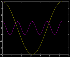
using a small value of h such as h=0.1 or 0.01.Example: Graphing the difference quotient:
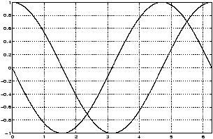
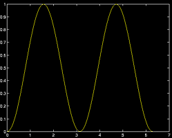
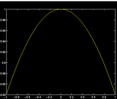
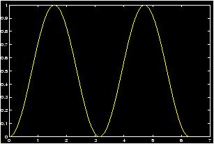
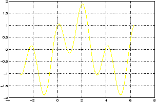
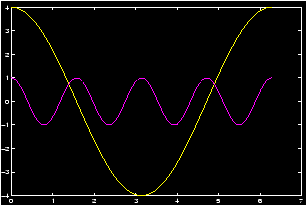
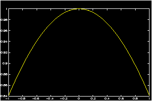
Let us create a plot of the derivative of f(x)=cos x over the interval [0,2p] based on the numerical evaluation of its difference quotient. We shall use h=0.01 in evaluating the difference quotient. The following MATLAB commands will plot both the function and its approximate derivative together.
>> h=0.01;
>> x=0:0.001:2*pi;                      % step size should be smaller
                                        % than h
>> difquo=(cos(x+h)-cos(x))./h;         % difference quotient
>> plot(x,cos(x),'r',x,difquo,'b'),grid % plot cos in red and difquo in blue
>> axis([0 2*pi -1 1])                  % a better frame for the
                                        %  graph
Here is another example which shows that we can reduce typing quite a bit, and hence possible errors.
Example: Baseball with wind correction
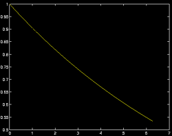
If there is constant acceleration, a baseball thrown from a height of x0 feet with an initial upward velocity of v0 feet/sec will fall according to the formula (0 Ł t Ł T).
y(t) = x0 + v0 t - 16 t2.
Here T is the time that the ball hits the ground.If we assume a slightly more realistic model, then the acceleration will depend upon the velocity of the baseball. A model for this yields the new formula for 0 Ł t Ł T.
| w(t) = x0 - 16 t + | ( | (16 + v0)/2 | ) | ( | 1 - e-2t | ) | . |
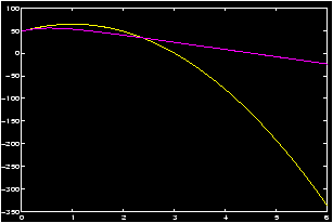
Let's suppose we want to follow the path of a baseball thrown from a fourth story window during the Yankees World Series Championship parade. Let x0 = 48, and v0 = 32.
-
Plot both functions y(t) and w(t) so that you can
determine from the graph the respective values of T.
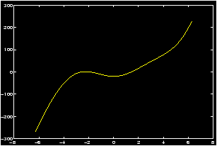
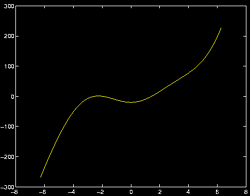
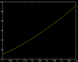
To find an estimate on the domain to plot the the two functions we note that the baseball under y(t) will hit the ground when the polynomial y = -16 t2 + 32 t + 48.>> roots([-16 32 48]) % find the zeroes ans = 3, -1 % actually a column vector
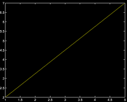
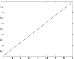
So T=3 for y(t) when the ball hits the ground. We expect the ball with wind-resistance to fall more slowly, so let's plot the functions over the interval [0,5].
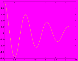
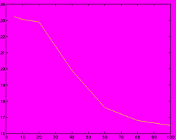
>> t = linspace(0,5); x0=48;v0=32;
>> y = -16*t.^2 + v0*t + x0;    % remember the .^
>> w = x0 - 16*t + (16+v0)/2 * ( 1 - exp(-2*t));
>> plot(t,y,t,w);
>> T = 4.5;                     % an approximation
We see that 4.5 is about correct for T for w(t).
Now answer questions about the ball with wind-resistance.
- What is the average velocity of the baseball
during [0,T].
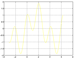
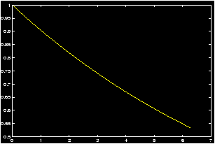
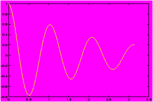
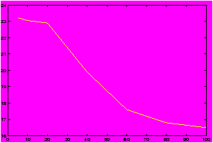
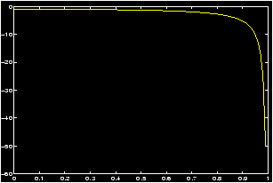
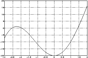
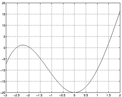
This is given by (w(T) - w(0))/T. To compute this without typing too much, let's use the up-arrow keys to give w. Notice w is defined for t = linspace(0,5) but we'll just redefine it to be T.>> t = 0; >> w0 = x0 - 16*t + (16+v0)/2 * ( 1 - exp(-2*t)); % use up arrow key, % and edit >> t = T; >> wT = x0 - 16*t + (16+v0)/2 * ( 1 - exp(-2*t)); % use up arrow key % and edit >> avg = (wT - w0)/T % pretty easy if done smartly - Let h= 0.1, plot the difference quotient of w(t) over the
interval [0,T].
We want to again use our definition of w(t) to minimize typing. Notice, we need to add an h in the right place.>> t = linspace(0,T); h = 0.1; >> w = x0 - 16*t + (16+v0)/2 * ( 1 - exp(-2*t)); % from up arrow >> wh = x0 - 16*(t+h) + (16+v0)/2 * ( 1 - exp(-2*(t+h))); % from up % arrow. >> difquo = (wh - w)/h; >> plot(t,difquo) - What is the time t when the ball is at
its highest point? What is the height?
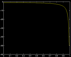
Using Calculus, we know this is when the derivative is 0, from the graph of the difference quotient this is t=1.
- The difference quotient is a good approximation to the
instantaneous velocity. From the graph, find the instantaneous
velocity when the ball hits the ground?
We see from the graph that it has a horizontal asymptote of -16. This says that the velocity stops decreasing after a certain amount. This is called a terminal velocity. From the graph it appears that T is big enough so that the ball is very near the terminal velocity, so we'll say the instantaneous velocity is -16 when the ball strikes the ground/
Concept: Implicit differentiation
Sometimes you are confronted with finding rates of change but you don't have a function relating x and y but rather an equation. That is y is implicitly defined in terms of x. The trick in mathematics is to take d/dx of both sides, use the chain rule properly and then solve for dy/dx in terms of x and y.
Using MATLAB to find numeric estimates requires a slightly different tack. Here is the main idea.
- Turn you equation into a problem involving level curves of a function: F(x,y) = c for some constant c.
- Differentiate using the chain rule:
Then solve to get
d dx F(x,y) = (Fx(x,y),Fy(x,y)) · (1, dy dx ) = 0 where Fx is the partial derivative in the x variable. We can use MATLAB to find this just as before because partial derivatives are just like regular derivatives of a function of a single variable.dy dx = - Fx(x,y) Fy(x,y)
|
(x2 - y6) = 2x - 6y5 |
|
= |
|
1 = 0 |
|
= |
|
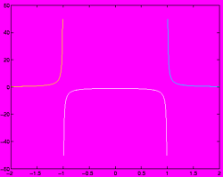
Using the difference quotient to estimate Fx and Fy we get instead the following. Suppose F(x,y) = x2 - 6y5 is defined in an m-file.
>> y0 = (1 - 1/4)^(1/6)
y0 = 0.95318
>> x0 = 1/2
x0 = 0.50000
>> h = .01
h = 0.010000
>> -(F(x0+h,y0) - F(x0,y0)) / (F(x0,y0+h) - F(x0,y0))
ans = -0.20839                  % this is the approximate value
>> (-2*x0)/(6*y0^5)
ans = -0.21182                  % this is the exact answer
The answer is not too far off and could be improved by using a smaller value of h. Notice that we used the secant line approximation for Fx and Fy
| Fx(x,y) » |
|
, Fy(x,y) » |
|
9.2 Symbolic derivatives