How are people getting high scores?

I spent a little while browsing the discussion forums on Kaggle, to pick up on tips, tricks and observations from the competitors.

• Reverse engineering the dataset structure
• Class weighting and de-duplication

Reverse engineering dataset

Turns out that values in the dataset are not unique! By reading the paper referenced in the competition, we can recover integer spectra for each row.

For each row, they take DNA of a bacterium, cut it into DNA substrings of length 10. Then a set of 100, 1'000, 100'000 or 1'000'000 of these substrings get processed and counted to produce the spectrum. This is normalized and de-biased.

So we could, say, re-introduce the bias and de-normalize it to get discrete predictor variables. And if we can tell how many decamers were used we could pay more attention to the more precise predictors.

Re-bias and de-normalize

def bias(w, x, y, z):
    return factorial(10) / (factorial(w) * factorial(x) * factorial(y) * factorial(z) * 4**10)

import re
hist_re = re.compile("A(\d+)T(\d+)G(\d+)C(\d+)")
biases = {col:bias(*[int(i) for i in hist_re.match(col).groups()]) for col in train.columns[:-1]}

train_i = pd.DataFrame({col: ((train[col] + biases[col]) * 1000000).round().astype(int) for col in train.columns[:-1]})
test_i = pd.DataFrame({col: ((test[col] + biases[col]) * 1000000).round().astype(int) for col in test.columns})
train_i

Detect small samples

Small samples have all entries a multiple of 10 or 1000. We add a "GCD" feature column to track this.

train['gcd'] = np.gcd.reduce(train_i, axis=1)
test['gcd'] = np.gcd.reduce(test_i, axis=1)

Dimensionality Reduction: PCA

A common method for visualizing complex datasets is principal component analysis. This method is also widely used for decorrelating features in datasets.

Correlation of variables can be calculated with the covariance matrix, given by the matrix multiplication formula $Cov(X) = (X-\mu_X)^T(X-\mu_X)$.

If we want decorrelated features, we want the covariance matrix to be diagonal. That is to say we want an orthonormal matrix $P$ such that $Cov(PX) = PCov(X)P^{-1}$ is diagonal. Such a $P$ will consist of the eigenvectors of $Cov(X)$.

These eigenvectors are called the principal components of $X$. Their corresponding eigenvalues measure the variance of that component. Geometrically we are finding a new basis for the space of our data such that the data spreads out most along the first axis, etc.

In sklearn

sklearn.decomposition.PCA implements PCA.

PCA as transformer

pca_pipeline = pipeline.make_pipeline(
  cleanup, decomposition.PCA(n_components=4), model)

PCA as visualizer

xy = decomposition.PCA(n_components=2).fit_transform(X)
scatter(xy[:,0],xy[:,1],c=y)

Let's look at the competition data!

xy = decomposition.PCA(n_components=2).fit_transform(train_i.drop(["gcd"]))
scatter(xy[:,0],xy[:,1],c=train_i["gcd"])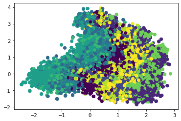

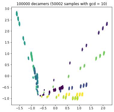
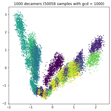
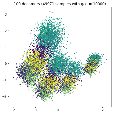
Let's look at the competition data!

Extract each separate value of GCD, plot in separate graphs, color by target.

Training separate classifiers for each GCD-value

from sklearn import pipeline, preprocessing, ensemble, model_selection
model_split = {g:pipeline.make_pipeline(preprocessing.StandardScaler(),
    ensemble.ExtraTreesClassifier()) for g in gcds}
for g in gcds:
    print(f"Model on GCD={g}, accuracy: {model_selection.cross_val_score(model_split[g], X_split[g], y_split[g], fit_params={'extratreesclassifier__sample_weight':wt_split[g]})}")

Model on GCD=10000, accuracy: [0.88503469 0.872481   0.86785596 0.86157912 0.81956378]
Model on GCD=1000, accuracy: [0.89768212 0.89139073 0.8787678  0.87512421 0.87247433]
Model on GCD=10, accuracy: [1. 0.99989341 1. 1. 1.]
Model on GCD=1, accuracy: [1. 1. 1. 1. 1.]

Training separate classifiers for each GCD-value

Full notebook ran for submission (including the cross-validation steps in the middle) in 240 seconds.

Submission accuracy: 0.95808 (setting n_estimators=300 nudged me up to 0.96942)

Lesson learned: ExtraTreesClassifier works well enough for GCD=1, GCD=10. More attention needed at GCD=1000, GCD=10000.