Neural Networks with Keras on TensorFlow

TensorFlow was the internal platform for the Google Brain team for AI and ML in research and production. In 2015, the platform was open source released under the Apache License.

Keras is a library for specifying neural network architectures. It was written by François Chollet and released in 2015. Until version 2.3, Keras supported a large array of computational backends, but Chollet was hired by Google and Keras integrated with and focused on Tensorflow 2.0.

In 2019, TensorFlow 2.0 was released, and re-cast the interface to the library to be primarily based on Keras, with the numpy-like tensor algebra of TensorFlow 1.0 de-emphasized.

TensorFlow has been adapted to run on everything from phones to compute clouds, with or without GPU acceleration. In 2016, Google released the TPU - a hardware accelerator that acts like a cluster of GPUs, optimized for AI and ML acceleration.

Coding for TensorFlow

To a large extent, TensorFlow mimics NumPy. Instead of np.array you use tf.Tensor as the fundamental unit. Very large parts of NumPy have been re-implemented, so that often you can just replace np. with tf.. When you do need a numpy array out, use x.numpy() to extract the numpy values.

Most of the time you will not be interacting on this deep layer. Instead, using the Keras interface, you can usually treat everything as if it was NumPy and scikit-learn.

Most of the differences come into play when you want to distribute computation, or get very detailed control of the computation.

Coding for Keras: Sequential or Functional

Keras has two basic approaches to defining a neural network:

• The Sequential Model: give a list of layers and data will flow through the list in the order you give.
• The Functional Model: each layer object acts like a function, and you define data flow by composing these functions.

The sequential model is easy to get started with, the functional model is far more flexible, and can do interesting things like multiple-input, multiple-output or shared-layer networks.

Coding for Keras: A Sequential CNN

Here is LeNet as a sequential Keras model:

model = tf.keras.Sequential([
  tf.keras.layers.Conv2D(6, (5,5), activation='sigmoid', 
    padding='same', input_shape=(28,28,1)),
  tf.keras.layers.AveragePooling2D((2,2), strides=2),
  tf.keras.layers.Conv2D(16, (5,5), activation='sigmoid'),
  tf.keras.layers.AveragePooling2D((2,2), strides=2),
  tf.keras.layers.Flatten(),
  tf.keras.layers.Dense(120, activation='sigmoid'),
  tf.keras.layers.Dense(84, activation='sigmoid'),
  tf.keras.layers.Dense(10, activation='softmax')
])

Coding for Keras: A Functional CNN

Here is LeNet as a functional Keras model (layer names follows Wikipedia):

inputs = tf.keras.Input((28,28,1))
C1 = tf.keras.Conv2D(6, (5,5), activation='sigmoid', 
                     padding='same')(inputs)
S2 = tf.keras.AveragePooling2D((2,2), strides=2)(C1)
C3 = tf.keras.Conv2D(16, (5,5), activation='sigmoid')(S2)
S4 = tf.keras.AveragePooling2D((2,2), strides=2)(C3)
F5 = tf.keras.Flatten()(S4)
D6 = tf.keras.Dense(120, activation='sigmoid')(F5)
D7 = tf.keras.Dense(84, activation='sigmoid')(D6)
outputs = tf.keras.Dense(10, activation='softmax')(D7)
model = tf.keras.Model(inputs=inputs, outputs=outputs)

Important Keras Layer Types

• Input - input layer for functional models
• Dense - classic, dense neural network layer
• Conv2D - convolutional layer
• AveragePooling2D - takes the average of a submatrix window that sweeps across the state matrix
• MaxPooling2D - takes the maximum of a submatrix window
• Dropout - randomly remove data (decreases overfitting)
• Reshape - reshape the matrix
• Normalization or BatchNormalization - preprocess to normalize variables
• Concatenate - combine several tensors to one
• CategoryEncoding, Discretization, TextVectorization, StringLookup - preprocessing to move between discrete and continuous data types

All the 2D layers also exist as 1D (sound, text) or 3D (video, volume data)).

Important Keras Activation Types

Keras implements a bunch of possible activation functions (the non-linearities that interleave with the linear forms):

• linear - do nothing
• sigmoid - classic $1/(1+e^{-x})$
• tanh - hyperbolic tangent
• relu - rectified linear unit (ReLU), make it leaky by setting the alpha parameter
• hard_sigmoid - linear approximation to sigmoid
• softplus - $\log(e^x+1)$, smooth differentiable approximation to ReLU
• softmax - makes a probability distribution

Coding for Keras: Compile

The code so far specifies a neural network model. To get it usable, we need more information - such as which optimizer to use, and what information we want to read out during training.

This is specified in the compile step:

model.compile(
    optimizer='rmsprop',
    loss='binary_crossentropy',
    metrics=[
        'accuracy',
        tf.keras.metrics.FalseNegatives(),
        tf.keras.metrics.FalsePositives(),
        'binary_crossentropy'
    ]
)

 Optimizers

• rmsprop
• sgd
• adagrad
• adadelta
• adam
• adamax

Also adaptive schedules in tf.keras.optimizers.schedules

Losses

• categorical_crossentropy, sparse_categorical_crossentropy - computes the cross entropy: a measure of shared information between probability distributions. Expects one-hot encoded data, the sparse_ version expects integer labels in a single variable.
• cosine_similarity - computes a normalized dot product, representing the cosine of the angle between the vectors. Scale-independent comparison of vectors, used a lot in text mining.
• mae, mape - mean average error, mean average percentage error
• mse, msle - mean squared error, mean squared log error

Metrics

• accuracy
• crossentropy
• FalsePositives
• FalseNegatives
• TruePositives
• TrueNegatives
• precision
• recall

Coding for Keras: Fit

Model training is very similar to scikit-learn

history = model.fit(X, y)

Important (new) parameters include:

• epochs - how many times do you loop through the entire dataset training?
• callbacks - a list of callback names or callback objects, to extract data while training
• validation_split - fraction of training data to automatically split out for validation
• validation_data - a tuple (X_val, y_val) to use for validation

Also new is that .fit returns a History object, that contains all the intermediate loss and metric values along the training sequence.

Callbacks

During training (and prediction, and model scoring) you can use callbacks to extract information as the process is running. These allow you to save periodic checkpoints, and to get running output on training metrics. Particularly interesting is the TensorBoard monitoring dashboard that was developed with TensorFlow. Callbacks live in tf.keras.callbacks.

• BackupAndRestore or ModelCheckpoint - save intermediate states to disk
• EarlyStopping - stop training when a particular metric has stopped improving
• LearningRateScheduler - adjust learning rates dynamically
• TensorBoard - output data to the TensorBoard visualizer
• LambdaCallback - wrap an arbitrary function as a callback

Coding for Keras: Predict

Just like in scikit-learn, use model.predict:

y_pred = model.predict(X)

 Calling a model

You can also get a prediction by using the model as a function-like object: y_pred = model(X). This is faster, but does not batch and does not scale. Most importantly, calling the model is differentiable and predict is not, so you can use model(X) to compute gradients and build training loops.

Coding for Keras: Evaluate

Scoring for Keras models does not use model.score like scikit-learn, but instead uses model.evaluate. This automatically batches computations and returns either a list of metrics (with names in model.metrics_names) or a dictionary (if you give the parameter return_dict=True)

scores = model.evaluate(X_val, y_val)

Coding for Keras: Saving and loading models

Something Keras does that scikit-learn does not do well is to save, transport and load models!

• model.save(filename) - save a model, weights and configuration and everything
• tf.keras.models.load_model(filename) - load a fully specified model from file
• model.to_json() and tf.keras.models.model_from_json(json_string) - save and load a model architecture to/from a JSON specification
• model.save_weights(filename), model.load_weights(filename) - save and load model parameters to and from a file

 Also important and new feature

The function model.summary will print out a string summarizing the network, with parameter counts and a data flow graph.

How to get started with TPU acceleration

We will be training some very large ML models in this competition. To help us, we are given access to TPU co-processors. These are packs of 8 cores, each of which is a GPU variant optimized for ML computations.

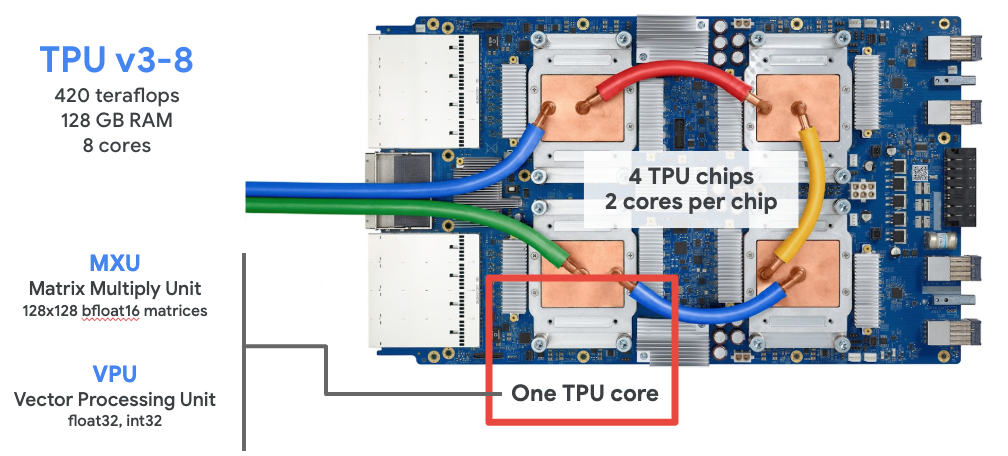
How to get started with TPU acceleration

The main benefit is that the typical neural network computations speed up significantly.

The main drawback is that there is quite a bit of boilerplate to setup everything to work smoothly with the new architecture. But all the boilerplate is written up in my public notebook - steal all you need from there!

We need to:

• Specify how to communicate with the TPU co-processor cluster
• Load Kaggle data through Google's cloud storage system
• Read the Tensorflow TFRecord data storage files

All this, and preferably in such a way that we can let the library optimize everything it could possibly optimize.

Communicating with the TPU cluster

We will create an object strategy that knows how to parallelize. Most often we won't need to interact with strategy, but when we specify our model we need to do this in a context given by strategy.scope().

try:
    tpu = tf.distribute.cluster_resolver.TPUClusterResolver()
    print(f"Running on TPU: ${tpu.master()}")
except ValueError:
    tpu = None

if tpu:
    tf.config.experimental_connect_to_cluster(tpu)
    tf.tpu.experimental.initialize_tpu_system(tpu)
    strategy = tf.distribute.experimental.TPUStrategy(tpu)
else:
    strategy = tf.distribute.get_strategy()

print(f"REPLICAS: {strategy.num_replicas_in_sync}")

Load Kaggle Data

We need to load data from the Google Cloud Storage (GCS) system. Kaggle has a package kaggle_datasets that knows how to connect Kaggle URLs to GCS URLs:

from kaggle_datasets import KaggleDatasets

GCS_DS_PATH = KaggleDatasets().get_gcs_path("tpu-getting-started")
print(GCS_DS_PATH)

IMAGE_SIZE = [192, 192] # or 224, 331, 512
GCS_PATH = f"{GCS_DS_PATH}/tfrecords-jpeg-{IMAGE_SIZE[0]}x{IMAGE_SIZE[1]}"

TRAINING_FILENAMES = tf.io.gfile.glob(f"{GCS_PATH}/train/*.tfrec")
VALIDATION_FILENAMES = tf.io.gfile.glob(f"{GCS_PATH}/val/*.tfrec")
TEST_FILENAMES = tf.io.gfile.glob(f"{GCS_PATH}/test/*.tfrec")

Read data from a TFRecord file

The data in this competition sits stored in specialized data containers called TFRecord files. To extract the data we need to provide a format specification ourselves, showing just how the data sits in the file. This works slightly differently for training data vs. test (and submission) data.

def read_labeled_tfrecord(example):
    LABELED_TFR_FORMAT = {
        "image": tf.io.FixedLenFeature([], tf.string),
        "class": tf.io.FixedLenFeature([], tf.int64)
    }
    example = tf.io.parse_single_example(example, LABELED_TFR_FORMAT)
    image = decode_image(example["image"])
    label = tf.cast(example["class"], tf.int32)
    return image, label

def read_unlabeled_tfrecord(example):
    UNLABELED_TFR_FORMAT = {
        "image": tf.io.FixedLenFeature([], tf.string),
        "id": tf.io.FixedLenFeature([], tf.string)
    }
    example = tf.io.parse_single_example(example, UNLABELED_TFR_FORMAT)
    image = decode_image(example["image"])
    idnum = example["id"]
    return image, idnum

Parse JPEG image data to Tensorflow tensors

We decode the JPEG-encoded image data, and while we're at it also rescale the entries so that instead of pixel intensities ranging 0-255, they range 0.0-1.0.

def decode_image(image_data):
    image = tf.image.decode_jpeg(image_data, channels=3)
    image = tf.cast(image, tf.float32)/255.0
    image = tf.reshape(image, [*IMAGE_SIZE,3])
    return image

Create a Dataset object

Tensorflow has extensive support for smart handling of datasets - where you give Tensorflow a list of files, and it automatically load-balances file reading, applies any post-processing steps you want to do, breaks the data up into batches, and provides everything in a format easy to read from other functions.

from tensorflow.data.experimental import AUTOTUNE
def load_dataset(filenames, labeled=True, ordered=False):
    ignore_order = tf.data.Options()
    if not ordered:
        ignore_order.experimental_deterministic = False # disable order, increase speed

    dataset = tf.data.TFRecordDataset(filenames, num_parallel_reads=AUTOTUNE)
    dataset = dataset.with_options(ignore_order)
    if labeled:
        dataset = dataset.map(read_labeled_tfrecord, num_parallel_calls=AUTOTUNE)
    else:
        dataset = dataset.map(read_unlabeled_tfrecord, num_parallel_calls=AUTOTUNE)
    return dataset

Setup data loading pipelines

We may want to do slightly different things with train, validation and test data. So we set up separate pipelines for creating each of these datasets.

def get_training_dataset():
    dataset = load_dataset(TRAINING_FILENAMES, labeled=True)
    dataset = dataset.map(data_augment, num_parallel_calls=AUTOTUNE)
    dataset = dataset.repeat()
    dataset = dataset.shuffle(2048)
    dataset = dataset.batch(BATCH_SIZE)
    dataset = dataset.prefetch(AUTOTUNE)
    return dataset

def get_validation_dataset(ordered=False):
    dataset = load_dataset(VALIDATION_FILENAMES, labeled=True, ordered=ordered)
    dataset = dataset.batch(BATCH_SIZE)
    dataset = dataset.cache()
    dataset = dataset.prefetch(AUTOTUNE)
    return dataset

def get_test_dataset(ordered=False):
    dataset = load_dataset(TEST_FILENAMES, labeled=False, ordered=ordered)
    dataset = dataset.batch(BATCH_SIZE)
    dataset = dataset.prefetch(AUTOTUNE)
    return dataset

Create data loading pipelines

Now that we have functions for creating the pipelines, we should use them too:

ds_train = get_training_dataset()
ds_val = get_validation_dataset()
ds_test = get_test_dataset(ordered=True) # to prepare for submissions

Make the model aware of the TPU

The last difference when coding for the TPU (instead of more "vanilla" Keras code) is how to create the model. This is done with a context manager to specify the parallelization strategy:

with strategy.scope():
    model = tf.keras.Sequential([
        tf.keras.layers.Conv2D(256, (4,4), activation='relu',
                               input_shape=[IMAGE_SIZE,3]),
        tf.keras.layers.MaxPooling2D((2,2)),
        tf.keras.layers.Conv2D(128, (4,4), activation='relu'),
        tf.keras.layers.MaxPooling2D((2,2)),
        tf.keras.layers.Conv2D(64, (4,4), activation='relu'),
        tf.keras.layers.MaxPooling2D((2,2)),
        tf.keras.layers.Conv2D(64, (4,4), activation='relu'),
        tf.keras.layers.MaxPooling2D((2,2)),
        tf.keras.layers.Flatten(),
        tf.keras.layers.Dense(128, activation='relu'),
        tf.keras.layers.Dense(len(CLASSES), activation='softmax')
    ])
model.summary()

Then compile, fit and predict as usual.

Code available in my sample notebook

The code in this presentation, and additional useful code for visualizing, for getting flower name labels, for preparing a submission can be found in my sample notebook:

https://www.kaggle.com/michiexile/mvj-first-sample-solution

I scored a macro F1-score of 0.22793 (harmonic mean of precision and recall) which places me at 99/135. You should be able to beat my results.