Gradient Descent

A Neural Network has the basic structure of interleaving linear maps and non-linear maps. Write $\sigma$ for the (differentiable) non-linearity - then:

\begin{multline*} \hat{y} = W^1 \sigma( W^2 \sigma( W^3 X + b^3) + b^2) + b^1 = \\ (W^1\bullet+b^1) \circ \sigma \circ (W^2\bullet+b^2) \circ \sigma \circ (W^3\bullet+b^1)(X) \end{multline*}

When training a neural network, we look for $W_1,\dots,W_k$ and $b_1,\dots,b_k$ that minimize some cost $C(\hat{y}(X_i), y_i)$.

Using the chain rule, we can take derivatives of the neural network with respect to each entry $W^d_{ij}$ and $b^d_i$. Compiling all these derivatives produces a gradient -- moving small steps in the direction opposite of the gradient moves us towards a local minimum.

Written out in detail, this produces the backpropagation algorithm

Backpropagation

Let's walk through a very small example:

$$ \hat{y} = (w^3\bullet+b^3) \circ \sigma \circ (w^2\bullet+b^2) \circ \sigma \circ (w^1\bullet+b^1)(X) $$

with one-dimensional states everywhere.

We are interested in the gradient of the cost function $\frac{\partial C}{\partial\bullet}$ wrt the 6 parameters.

Backpropagation

$$ \hat{y} = (w^3\bullet+b^3) \circ \sigma \circ (w^2\bullet+b^2) \circ \sigma \circ (w^1\bullet+b^1)(X) $$

Write $a^j$ for the activation at each stage and $z^j = w^ja^{j-1}+b^j$ for the input to the non-linearity.

$$ \frac{\partial C}{\partial w^3} = \frac{\partial C}{\partial a^3}\frac{\partial a^3}{\partial z^3}\frac{\partial z^3}{\partial w^3} = C'(a^3)\cdot\sigma'(z^3)\cdot a^{2} $$$$ \frac{\partial C}{\partial b^3} = \frac{\partial C}{\partial a^3}\frac{\partial a^3}{\partial z^3}\frac{\partial z^3}{\partial b^3} = C'(a^3)\cdot\sigma'(z^3)\cdot 1 $$$$ \frac{\partial C}{\partial a^2} = \frac{\partial C}{\partial a^3}\frac{\partial a^3}{\partial z^3}\frac{\partial z^3}{\partial a^2} = C'(a^3)\cdot\sigma'(z^3)\cdot w^3 $$

Backpropagation

$$ \hat{y} = (w^3\bullet+b^3) \circ \sigma \circ (w^2\bullet+b^2) \circ \sigma \circ (w^1\bullet+b^1)(X) $$

Write $a^j$ for the activation at each stage and $z^j = w^ja^{j-1}+b^j$ for the input to the non-linearity.

$$ \frac{\partial C}{\partial w^2} = \frac{\partial C}{\partial a^2}\frac{\partial a^2}{\partial z^2}\frac{\partial z^2}{\partial w^2} = \color{blue}{w^3C'(a^3)\cdot\sigma'(z^3)}\cdot\sigma'(z^2)\cdot a^{1} $$$$ \frac{\partial C}{\partial b^2} = \frac{\partial C}{\partial a^2}\frac{\partial a^2}{\partial z^2}\frac{\partial z^3}{\partial b^2} = \color{blue}{w^3C'(a^3)\cdot\sigma'(z^3)}\cdot\sigma'(z^2)\cdot 1 $$$$ \frac{\partial C}{\partial a^1} = \frac{\partial C}{\partial a^2}\frac{\partial a^2}{\partial z^2}\frac{\partial z^2}{\partial a^1} = \color{blue}{w^3C'(a^3)\cdot\sigma'(z^3)}\cdot\sigma'(z^2)\cdot w^2 $$

Backpropagation

As we step up to higher-dimensional activations, most of this stays the same - when calculating $\partial C / \partial a$ for the dependency on activations in previous layers, we need to sum across all the activations it contributes to.

\begin{align*} \frac{\partial C}{\partial w^d_{jk}} &= a^{d-1}_k\sigma'(z^d_j)\frac{\partial C}{\partial a^d_j} \\ \frac{\partial C}{\partial b^d_{j}} &= \sigma'(z^d_j)\frac{\partial C}{\partial a^d_j} \\ \frac{\partial C}{\partial a^d_j} &= \sum w^{d+1}_{jk}\sigma'(z^{d+1}_j)\frac{\partial C}{\partial a^{d+1}_j} &\text{ or }& 2(a^L_j-y_j) \end{align*}

Images have structure

The dense network layers assume that all input features are structureless: systematic correlations are not used.

For images, this means that the result will depend on where in the image an object exists.

Below, we have evaluation scores for

1. The MNIST test set
2. The MNIST test set, offset by 2 pixels up and 2 pixels left

model.evaluate(X_val, y_test), model.evaluate(X_test, y_test)

313/313 [==============================] - 4s 11ms/step - loss: 0.5601 - accuracy: 0.9443
313/313 [==============================] - 4s 12ms/step - loss: 73.6791 - accuracy: 0.2102

([0.5601367950439453, 0.9442999958992004],
 [73.67906188964844, 0.2101999968290329])

Translation Invariance

The result of a classifier should preferably not depend on where in the image a particular object exists; treating pixels as completely different the way that the dense network does is not a stable solution.

There are several ways to deal with this:

1. Extend training set: train on various offsets and transformations of the original training element. This way, the network sees a wider range of inputs and can adapt.
2. Convolutional Layers

Convolutional Layers

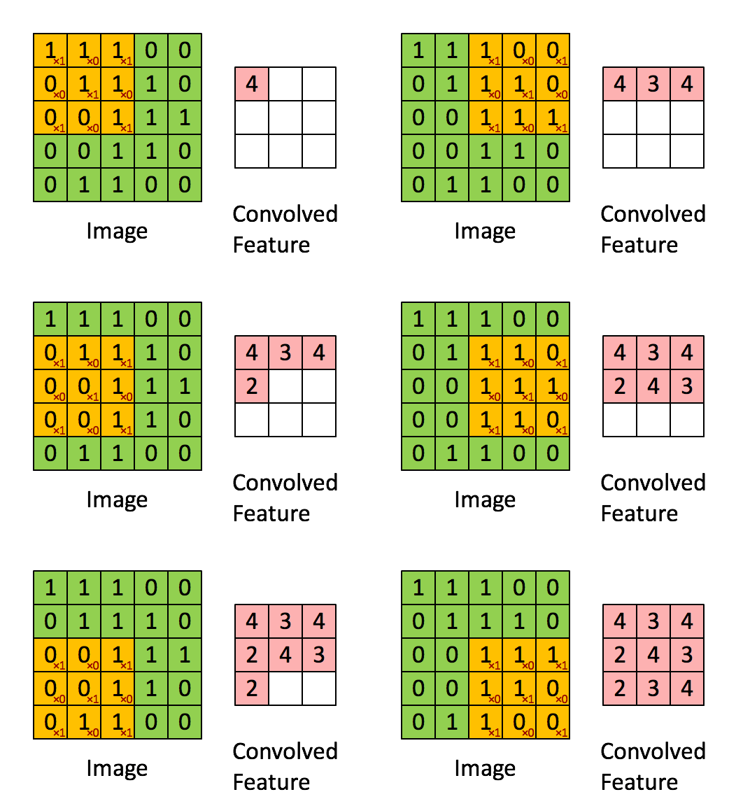
In a convolutional layer, a smaller layer is applied repeatedly to blocks of cells, and the outputs are collected in a matrix (cube) of outputs.

Convolutional Layers

Some important terminology:

• kernel - the moving window. 3x3 is a common size for small images
• stride - how many pixels the window moves for each step
• filter - a single output dimension from the network

A convolutional layer shrinks the image, but by using many filters encodes abstractions about the image.

It is common to see features like edges encoded in early convolutional layers, and higher level features in later layers.

Convolutional Layers

Since the same network layer is trained on each kernel window, the spatial dependency that broke our dense network earlier is less of an issue.

fig_1

fig_2

fig_03

fig_1

fig_2

fig_13

By the end of all the reductions, the two digits come out quite different.

fig_03

fig_13

For practical applications

There are several strong visual networks already available. Some examples are:

• LeNet (1990s; LeCun; reads digits)
• AlexNet (won the ImageNet ILSVRC challenge in 2012)
• ZF Net (won the ILSVRC challenge in 2013)
• GoogLeNet (won the ILSVRC challenge 2014; added the inception module)
• VGGNet (second place in ISLVRC 2014)
• ResNet (won the ILSVRC challenge 2015) - currently state of the art architecture

One way these can be used is to use most of the network as a feature extractor, and then add your own final layer that you train on your own task.