Categorical Data

Mikael Vejdemo-Johansson

Red thread of today

Last Lecture was all about how to show Goodness of Fit - whether or not some set of observations adhere to some pre-specified probability distribution.

Today’s Lecture is about several different questions that boil down to the exact same computational setup and exact same answer.

We are interested $I$ populations, and within each classify observations as one of $J$ different categories. We count how many occurrences each category has in each population.
We are interested in a single population, but classify observations twice with respect to two different sets of categories. The first factor has $I$ categories, and the second factor has $J$ categories. We count occurrences of each pair of observed categories.

Notice that 1. can be re-interpreted as 2. if we let the population be the union of each subpopulation, and mark each observation with its population of origin.

Some notation

In each of the two scenarios, we can compile our counts into a rectangular table with $I$ rows and $J$ columns. We shall write, using the observation that subpopulation can be seen as another factor:


$n=n_{,}=\sum_{i=1}^I\sum_{j=1}^J n_{i,j}$	total number of observations
$n_{i,j}$	The count of occurrences of the $j$th category paired with the $i$th category
$n_{*,j}=\sum_{i=1}^I n_{ij}$	the count of occurrences of the $j$th category
$n_{i,*}=\sum_{j=1}^Jn_{i,j}$	the count of occurrences of the $i$th category
$p_{i,j}=n_{i,j}/n_{,}$	overall proportion of observation in the $i,j$ cell
$p_{j\|i}=n_{i,j}/n_{i,*}$	proportion of observations with the $i$th category that fall into category $j$.
$p_{i,}=n_{i,}/n_{,}$	proportion of occurrences of category $i$ in the entire dataset
$p_{,j}=n_{,j}/n_{,}$	proportion of occurrences of category $j$ in the entire population

Two different questions

In Scenario 1., we would primarily be interested in testing for homogeniety. The null hypothesis is that each category $j$ has the same prevalence in each population, so that $p_{1,j}=p_{2,j}=\dots=p_{I,j}$.

When this null hypothesis is true, we can expect $p_{j|i}=p_{*,j}$ for all $i,j$. Hence, the expected count for the $i,j$ cell would be $\EE[n_{i,j}] = n_{i,*}\cdot p_{*,j}$. Using $\hat p_{*,j}=n_{*,j}/n_{*,*}$, we get a simple formula for the expected counts:

\[ \hat e_{i,j} = n_{i,*}\cdot{n_{*,j}\over n_{*,*}} = {(i\text{th row total})\cdot(j\text{th column total})\over \text{total count}} \]

Two different questions

In Scenario 2., we would primarily be interested in independence: does the first factor and the second factor influence each other, or are the two discrete random variables independent from each other.

We can estimate the probability of observing category $i$ in the first factor as $p_{i,*}=\sum_{j}p_{i,j}$, and of category $j$ in the second factor as $p_{*,j}=\sum_ip_{i,j}$.

If [observing category $i$ in the first factor] is independent from [observing category $j$ in the second factor], we would expect the joint probability to be the product of individual probabilities. Hence:

\[ \hat e_{i,j} = n\cdot\hat p_{i,*}\cdot\hat p_{*,j} = \color{DarkMagenta}{n}\cdot{n_{i,*}\over \color{DarkMagenta}{n}}\cdot{n_{*,j}\over n} = {(i\text{th row total})\cdot(j\text{th column total})\over \text{total count}} \]

Degrees of Freedom

We know how to get expected counts in both scenarios - and come up with the exact same formula in both cases. So we have expected counts and observed counts - it’s a multinomial setup! Pearson’s Theorem applies!

How many degrees of freedom do we need though?

Scenario 1: Each row has $J-1$ freely determined cell counts (for fixed $n_{i,*}$), so we get $I(J-1)$ freely determined cells. We estimate $J$ parameters $p_{*,1},\dots,p_{*,J}$, but these parameters sum to 1, so only $J-1$ of them are independent. The estimated parameters lower our DoF from $I(J-1)$ to $I(J-1)-(J-1)=\boxed{(I-1)(J-1)}$.

Scenario 2: We have $IJ$ cell counts, but a fixed total count $n$, yielding $IJ-1$ freely determined cell counts. We estimate $I$ different $p_{i,*}$ and $J$ different $p_{*,j}$, but each of the sets need to sum to 1, so we estimate $I-1$ and $J-1$ independent parameters. The total count and each estimated parameter lowers DoF by 1, yielding $IJ-1-(I-1)-(J-1) = IJ-I-J+1 = \boxed{(I-1)(J-1)}$.

Homogeniety is about independence

The homogeniety claim says that no matter what the subpopulation is, the proportions of each observed category are the same.

In other words, knowledge about the subpopulation does not influence the proportions of the observed categories.

Hence, the homogeniety question really is a question of independence, with the subpopulation membership tagged as a different observed factor.

Note also that \[ p_{i,j} = {n_{i,j}\over n_{*,*}} = {n_{i,j}\over n_{i,*}}\cdot{n_{i,*}\over n_{*,*}} = p_{j|i}\cdot p_{i,*} \]

Chi-square Test of Independence

Test of Independence for a 2-way Contingency Table

Null Hypothesis: $p_{i,j} = p_{i,*}\cdot p_{*,j}$, or equivalently all $p_{j|i} = p_{j|i'}$.
Test Statistic: Write $E_{i,j}={n_{i,*}\cdot n_{*,j}\over n_{*,*}}$, and $O_{i,j}$ for the observed count in cell $i,j$.; $X=\sum_i\sum_j {(O_{i,j}-E_{i,j})^2\over E_{i,j}}$
Rejection Region: $X\geq \chi^2_{\alpha, (I-1)(J-1)}$
p-values: $1-CDF_{\chi^2((I-1)(J-1))}(X) = SF_{\chi^2((I-1)(J-1))}(X)$
Sample Size Condition: $E_{i,j}\geq 5$ for all cells.

Example

Exercise 13.28

6 different populations of fruitflies with different male genotypes were studied for the sex combinations of two recombinants. The question is whether data supports a hypothesis that the frequency distribution among the three combinations is homogenous with respect to the genotypes.

Code

df = tibble(
  genotype=rep(c(1,2,3,4,5,6), each=3) %>% as.character %>% fct,
  sexcombination=fct(rep(c("MM","MF","FF"), times=6)),
  counts=c(35,80,39,
           41,84,45,
           33,87,31,
           8 ,26,8 ,
           5 ,11,6 ,
           30,65,20
           )
)
tbl = xtabs(counts ~ genotype+sexcombination, data=df)
tbl %>% kable(row.names=T)

	MM	MF	FF
1	35	80	39
2	41	84	45
3	33	87	31
4	8	26	8
5	5	11	6
6	30	65	20

Example

Exercise 13.28

With margin.table in R we can get total and margin counts:

Code

tbl %>% margin.table(1) %>% kable
tbl %>% margin.table(2) %>% kable
tbl %>% margin.table() %>% kable

genotype	Freq
1	154
2	170
3	151
4	42
5	22
6	115

sexcombination	Freq
MM	152
MF	353
FF	149

x
654

Example

Exercise 13.28

$H_0:$ The sexcombination proportions are independent of the genotype label.

$H_a:$ The sexcombination proportions are dependent on the genotype label.

Example

Exercise 13.28

We can get the products $n_{i,*}\cdot n_{*,j}$ easily using the margin.table function and matrix multiplication (using %*% in R). We use t to transpose one of the vectors:

Code

ni.nj = margin.table(tbl, 1) %*% t(margin.table(tbl, 2)) 
ni.nj %>% kable(row.names=T, caption="Products of marginal counts")
expected = ni.nj / margin.table(tbl)
expected %>% kable(row.names=T, digits=1, caption="Expected counts")
differences = tbl - expected
differences %>% kable(row.names=T, digits=1, caption="Deviations")

Products of marginal counts
	MM	MF	FF
1	23408	54362	22946
2	25840	60010	25330
3	22952	53303	22499
4	6384	14826	6258
5	3344	7766	3278
6	17480	40595	17135

Expected counts
	MM	MF	FF
1	35.8	83.1	35.1
2	39.5	91.8	38.7
3	35.1	81.5	34.4
4	9.8	22.7	9.6
5	5.1	11.9	5.0
6	26.7	62.1	26.2

Deviations
	MM	MF	FF
1	-0.8	-3.1	3.9
2	1.5	-7.8	6.3
3	-2.1	5.5	-3.4
4	-1.8	3.3	-1.6
5	-0.1	-0.9	1.0
6	3.3	2.9	-6.2

Example

Exercise 13.28

Code

residuals = differences / sqrt(expected)
chisq.terms = residuals^2

differences %>% kable(row.names=T, digits=1, caption="Deviations")
residuals %>% kable(row.names=T, digits=1, caption="Residuals")
chisq.terms %>% kable(row.names=T, digits=1, caption="Chi-square terms")

Deviations
	MM	MF	FF
1	-0.8	-3.1	3.9
2	1.5	-7.8	6.3
3	-2.1	5.5	-3.4
4	-1.8	3.3	-1.6
5	-0.1	-0.9	1.0
6	3.3	2.9	-6.2

Residuals
	MM	MF	FF
1	-0.1	-0.3	0.7
2	0.2	-0.8	1.0
3	-0.4	0.6	-0.6
4	-0.6	0.7	-0.5
5	-0.1	-0.3	0.4
6	0.6	0.4	-1.2

Chi-square terms
	MM	MF	FF
1	0.0	0.1	0.4
2	0.1	0.7	1.0
3	0.1	0.4	0.3
4	0.3	0.5	0.3
5	0.0	0.1	0.2
6	0.4	0.1	1.5

Example

Exercise 13.28

We sum up the chi-square terms to find a test statistic of 6.4625306.

With 3 sex combinations and 6 genotypes, we get $(6-1)\cdot(3-1)=5\cdot2=10$ degrees of freedom.

Hence, using pchisq(sum(chisq.terms), 10, lower.tail=FALSE) we get a p-value of 0.7750229.

This means that the observed data does not contain compelling evidence of a departure from a homogeniety null hypothesis: it is reasonable to believe that the data could have been from 6 homogenously distributed populations.

Example

Exercise 13.29

A random sample of high school and college students were asked about political views and about marijuana usage, resulting in the following data:

Code

df = tibble(
  political=rep(c("Liberal","Conservative","Other"), each=3) %>% fct,
  marijuana=rep(c("Never", "Rarely", "Frequently"), times=3) %>% fct,
  counts=c(479,173,119,
           214, 47, 15,
           172, 45, 85)
)
tbl = xtabs(counts ~ political+marijuana, data=df)
tbl %>% kable(row.names = T)

	Never	Rarely	Frequently
Liberal	479	173	119
Conservative	214	47	15
Other	172	45	85

Example

Exercise 13.29

Are political views and marijuana usage independent? A chisquared test of independence is appropriate.

$H_0:$ Political views and marijuana usage are independent.

$H_a:$ There is a statistically significant dependency between political views and degrees of marijuana usage.

Example

Exercise 13.29

We get marginal counts:

Code

tbl %>% margin.table(1) %>% kable
tbl %>% margin.table(2) %>% kable
tbl %>% margin.table() %>% kable

political	Freq
Liberal	771
Conservative	276
Other	302

marijuana	Freq
Never	865
Rarely	265
Frequently	219

x
1349

Example

Exercise 13.29

With the same vector multiplication, we get expected counts, deviations and residuals.

Code

expected = (margin.table(tbl, 1) %*% t(margin.table(tbl, 2)))/margin.table(tbl)
differences = tbl - expected
residuals = differences/sqrt(expected)
chisq.terms = residuals^2

expected %>% kable(row.names=T, digits=1, caption="Expected")
differences %>% kable(row.names=T, digits=1, caption="Deviations")
residuals %>% kable(row.names=T, digits=1, caption="Residuals")
chisq.terms %>% kable(row.names=T, digits=1, caption="Chi-square terms")

Expected
	Never	Rarely	Frequently
Liberal	494.4	151.5	125.2
Conservative	177.0	54.2	44.8
Other	193.6	59.3	49.0

Deviations
	Never	Rarely	Frequently
Liberal	-15.4	21.5	-6.2
Conservative	37.0	-7.2	-29.8
Other	-21.6	-14.3	36.0

Residuals
	Never	Rarely	Frequently
Liberal	-0.7	1.8	-0.6
Conservative	2.8	-1.0	-4.5
Other	-1.6	-1.9	5.1

Chi-square terms
	Never	Rarely	Frequently
Liberal	0.5	3.1	0.3
Conservative	7.7	1.0	19.8
Other	2.4	3.5	26.4

Example

Exercise 13.29

These chi-squared terms sum up to 64.6541702.

With 3 political labels, and 3 levels of marijuana usage we get $(3-1)\cdot(3-1)=4$ degrees of freedom.

This yields a p-value of $3.0431451\times 10^{-13}$.

A reasonable conclusion is to summarily reject the null hypothesis of independence. The degree to which students smoke marijuana and their political views are not independent.

Ordinal Variables and Logistic Regression

Exercise 13.25, 13.34

The text book suggests that if one of the variables in a contingency table is ordinal, we can use ranks to treat that variable as numeric and use logistic regression for similar purposes to the chi-squared tests we developed. This approach can be more sensitive than a chi-squared approach.

An experiment studies the effects of leaf removal on a particular plant’s ability to mature its fruits. The following counts were collected:

Code

mature = tibble(
  leaves.removed = c(0, 2, 4, 6, 8),
  matured = c(141,28,25,24,20),
  aborted = c(206,69,73,78,82)
)

mature %>% t %>% kable

leaves.removed	0	2	4	6	8
matured	141	28	25	24	20
aborted	206	69	73	78	82

Ordinal Variables and Logistic Regression

Exercise 13.25, 13.34

A chi-squared test can be performed - either using the formulas we have been using, or using ready-made functions: scipy.stats.chisquare in Python or with chisq.test in R. The Python function requires a lot more detailed handling to do the right thing (adjusting Degrees of Freedom, pre-computing expected counts).

Code

mature.chisq = chisq.test(mature %>% select(matured, aborted))
mature.chisq


    Pearson's Chi-squared test

data:  mature %>% select(matured, aborted)
X-squared = 24.821, df = 4, p-value = 5.467e-05

This p-value allows us to reject the null hypothesis of independent variables and conclude that there is some relation between how many leaves were removed and the probability of a fruit maturing.

Ordinal Variables and Logistic Regression

Exercise 13.25, 13.34

The suggested alternate approach would take the number of leaves removed (…or their rankings) as predictor, and predict the probability of maturation. We augment the data:

Code

mature$p.mature = with(mature, matured/(matured+aborted))
mature$predictor = rank(mature$leaves.removed)

mature %>% t %>% kable

leaves.removed	0.0000000	2.0000000	4.000000	6.0000000	8.0000000
matured	141.0000000	28.0000000	25.000000	24.0000000	20.0000000
aborted	206.0000000	69.0000000	73.000000	78.0000000	82.0000000
p.mature	0.4063401	0.2886598	0.255102	0.2352941	0.1960784
predictor	1.0000000	2.0000000	3.000000	4.0000000	5.0000000

Ordinal Variables and Logistic Regression

Exercise 13.25, 13.34

Now we can use glm in R to perform the logistic regression calculations. If we predict proportions of successes, we have to give the number of trials as weights:

Code

mature.glm = glm(p.mature ~ predictor, family=binomial(), data=mature, weights=with(mature,matured+aborted))
summary(mature.glm)


Call:
glm(formula = p.mature ~ predictor, family = binomial(), data = mature, 
    weights = with(mature, matured + aborted))

Deviance Residuals: 
      1        2        3        4        5  
 0.4395  -0.9348  -0.4708   0.2255   0.3523  

Coefficients:
            Estimate Std. Error z value Pr(>|z|)    
(Intercept) -0.15913    0.14439  -1.102     0.27    
predictor   -0.26810    0.05691  -4.711 2.47e-06 ***
---
Signif. codes:  0 '***' 0.001 '**' 0.01 '*' 0.05 '.' 0.1 ' ' 1

(Dispersion parameter for binomial family taken to be 1)

    Null deviance: 25.2534  on 4  degrees of freedom
Residual deviance:  1.4636  on 3  degrees of freedom
AIC: 30.715

Number of Fisher Scoring iterations: 3

The z-test p-value tells us that the hypothesis of no relationship (ie slope $\beta_1=0$) can be rejected.

Notice that the p-values differ: $5.4666654\times 10^{-5}$ for the chi-squared test, and $2.4677126\times 10^{-6}$ for the logistic regression.

Your Homework

12:7 - Victoria Paukova

$y = f(x) = 1800 + 1.3x$

a.: $\EE[Y]$ when $x=2500$? $f(2500) = 5050$.

b.: The change in 28-day strength (y) with an increase in accelerated strength (x) of 1 will be 1.3, since that is the slope.

c.: The change in 28-day strength (y) with an increase in accelerated strength (x) of 100 will be 130.

d.: The change in 28-day strength (y) with an decrease in accelerated strength (x) of 100 will be -130.

12:8 - Victoria Paukova

$y = f(x) = 1800 + 1.3x$, $\epsilon = 350 psi$

a.: Probability of $y>5000 psi$ when $x=2000$

\[ \PP(Y > 5000 | x=2000) = \PP\left(Z>{5000 - (1800+1.3\cdot 2000)\over 350}\right) = \PP(Z>1.714) \approx.04326 \]

b.: Probability of $y>5000 psi$ when $x=2500$

\[ \PP(Y > 5000 | x=2500) = \PP\left(Z>{5000 - (1800+1.3\cdot 2500)\over 350}\right) = \PP(Z>-0.1429) \approx 0.5568 \]

c.: First observation when $x=2000$, second when $x=2500$. What’s the probability of the second result exceeding the first by more than 1000?

\[ Y_1 = 4400, Y_2 = 5050, \EE[Y_2-Y_1] = 650 \\ \PP(Y_2-Y_1>1000) = \PP\left(Z>{1000-650\over\sqrt{2\cdot 350^2}}\right) \approx \PP(Z>0.7071) \approx 0.23975 \]

12:8 d. - Maxim Kleyer

\[ \EE[Y_2-Y_1] = \EE[(1800+1.3x_2)-(1800+1.3x_1)] = 1.3\cdot(x_2-x_1) \]

\[ \begin{align*} \PP(Y_2-Y_1>0) &= .95 \\ \PP\left(Z>{0-1.3\cdot(x_2-x_1)\over\sqrt{2\cdot 350^2}}\right) &= .95 \\ \PP\left(Z < -{-1.3\cdot(x_2-x_1)\over\sqrt{245000}}\right) &= .95 \\ \PP(Z<1.645) &= .95 & \color{DarkMagenta}{\text{from the inverse CDF}} \\ {1.3\cdot(x_2-x_1)\over 494.97} &\approx 1.645 \\ 1.3\cdot(x_2-x_1) &\approx 814.2236 \\ x_2-x_1 &\approx 626.3274 \end{align*} \]

12:20 - Justin Ramirez

a.: $\beta_0$ is given as the constant $coef = 0.365$. $\beta_1$ is given as the no3 depo $coef=0.966$

b.: at $x=0.5$, $\hat y=0.365+0.966\cdot0.5\Rightarrow0.848$

c.: The SS error given is 0.4106.

$\hat\sigma = se(e) = \sqrt{V(e)}$. $V(e)=SSe/(n-2)=0.4106/11\approx0.0373$

$\hat\sigma = \sqrt{0.0373} \approx 0.193$

d.: The total variation is given as 1.4533. The model given shows that the 69.2%.

12:52 e.- Victoria Paukova

The regression equation is lichen 
N = 0.365 + 0.967 no3 depo

Predictor  Coef    Stdev   t-ratio  P
Constant   0.36510 0.09904 3.69   0.004
no3 depo   0.9668  0.1829  5.29   0.000

S = 0.1932  R-sq = 71.7%  R-sq (adj) = 69.2%

Analysis of Variance
Source     DF   SS     MS     F    P 
Regression  1 1.0427 1.0427 27.94 0.000
Error      11 0.4106 0.0373
Total      12 1.4533

A 95% CI vs PI for N when NO3- = .5, and then for NO3-=.8

\[ CI: \hat Y \pm t_{\alpha/2,n-2}\cdot S_{\hat Y} \qquad PI: \hat Y \pm t_{\alpha/2,n-2}\cdot \sqrt{S^2 + S_{\hat Y}^2} \\ S_{\hat Y} = S\sqrt{{1\over n}+{(x^*-\overline x)^2\over S_{xx}}} \]

In both of these equations, the actual width of the interval only depends on the part that comes after $\pm$. Since we are working with the same $\alpha$ and same degrees of freedom, the only difference comes from the different $x^*$ values. Since both formulas have $x^*$ in the numerator, the CI for NO3-=.8 should be slightly wider than for NO3-=.5. We also know that the PI’s are going to be wider than the CI’s, as evident from the formulas above.

12:60 - Maxim Kleyer

Correlation coefficient $\Rightarrow r = .449$

a.: $H_0:\rho=0$, $H_a:\rho\neq0$, $\alpha=.05$

\[ t = {r\sqrt{n-2}\over\sqrt{1-r^2}} \Rightarrow {0.449\sqrt{14-2}\over \sqrt{1-(.449)^2}} \approx {1.5554 \over 0.8935} \approx 1.7407 \]

p-values = TDIST(1.7407, 12, 2) (Excel command) $\approx 0.10729$.

b.: $r^2 = (0.449)^2 .2017 = $ 20.17% of observations can be explained using linear regression model

MVJ: It’s not really that some of the observations are explained and others are not explained - it is that the variation decomposes into variation due to the regression model and variation due to noise, and that the variation due to the regression constitutes about 20.17% of the total variation in the data.

12:74 - Victoria Paukova

Code

library(tidyverse)
library(foreach)
library(ggplot2)
df = tibble(HR=c(43.5,44,44,44.5,44,45,48,49,49.5,51,54.5,57.5,57.7,61,63,72),
            VO=c(22,21,22,21.5,25.5,24.5,30,28,32,29,38.5,30.5,57,40,58,72))

ggplot(df, aes(x=HR, y=VO)) + 
  geom_point() +
  labs(x="HR", y="VO2")
summary(df)
ggplot(df, aes(sample=HR)) + 
  geom_qq() + geom_qq_line() +
  labs(title="Probability Plot")
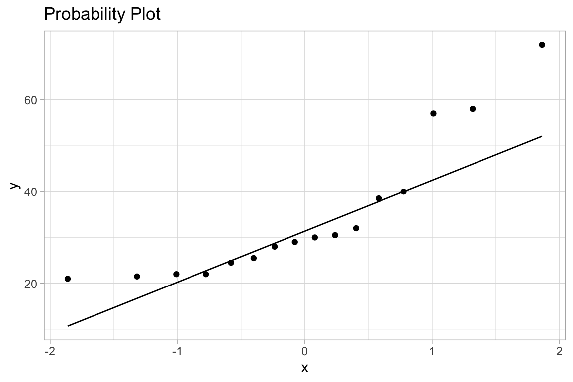
ggplot(df, aes(sample=VO)) + 
  geom_qq() + geom_qq_line() +
  labs(title="Probability Plot")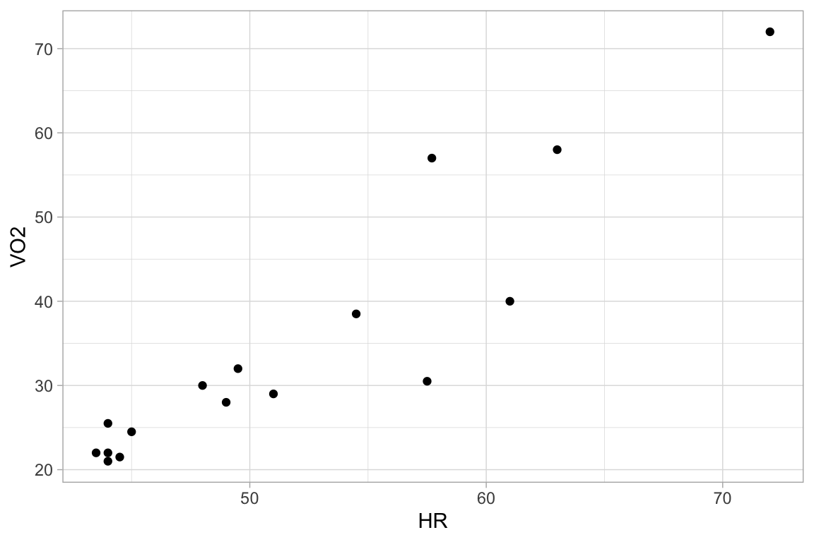

       HR              VO       
 Min.   :43.50   Min.   :21.00  
 1st Qu.:44.38   1st Qu.:23.88  
 Median :49.25   Median :29.50  
 Mean   :51.76   Mean   :34.47  
 3rd Qu.:57.55   3rd Qu.:38.88  
 Max.   :72.00   Max.   :72.00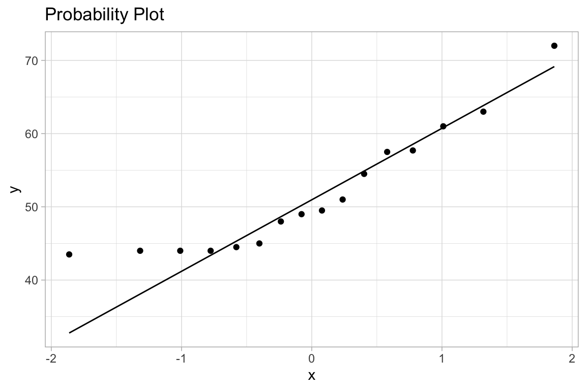

12:74 - MVJ

For the linear regression itself, we compute and graph:

Code

library(broom)

model = lm(VO ~ HR, data=df)
model.a = augment(model)
summary(model)
ggplot(model.a, aes(x=HR)) + 
  geom_point(aes(y=VO)) +
  geom_line(aes(y=.fitted)) + 
  labs(title="Fitted line and data")
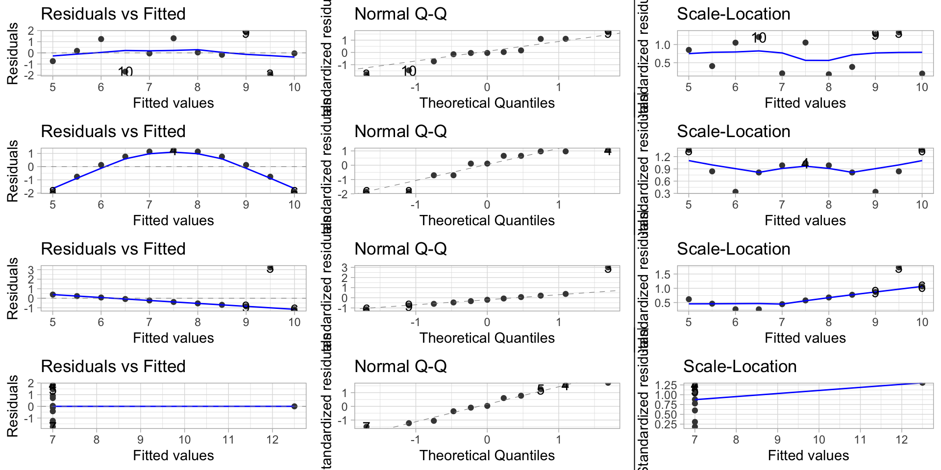
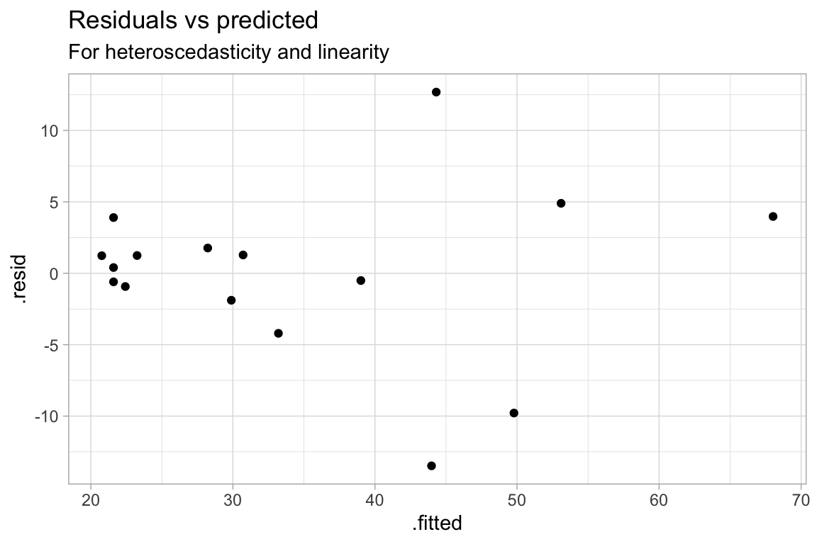
ggplot(model.a, aes(.fitted, .resid)) +
  geom_point() +
  labs(title="Residuals vs predicted", subtitle="For heteroscedasticity and linearity")
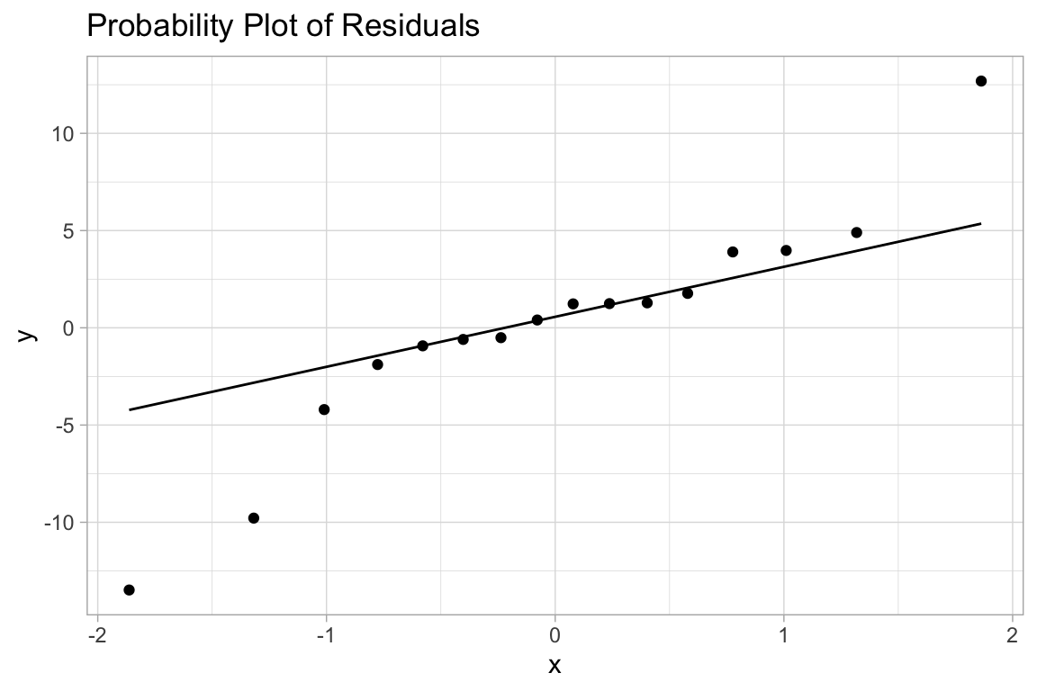
ggplot(model.a, aes(sample=.resid)) +
  geom_qq() + geom_qq_line() +
  labs(title="Probability Plot of Residuals")


Call:
lm(formula = VO ~ HR, data = df)

Residuals:
     Min       1Q   Median       3Q      Max 
-13.4817  -1.1676   0.8162   2.3026  12.6867 

Coefficients:
            Estimate Std. Error t value Pr(>|t|)    
(Intercept) -51.3547     9.7949  -5.243 0.000124 ***
HR            1.6580     0.1869   8.871 4.03e-07 ***
---
Signif. codes:  0 '***' 0.001 '**' 0.01 '*' 0.05 '.' 0.1 ' ' 1

Residual standard error: 6.119 on 14 degrees of freedom
Multiple R-squared:  0.849, Adjusted R-squared:  0.8382 
F-statistic: 78.69 on 1 and 14 DF,  p-value: 4.032e-07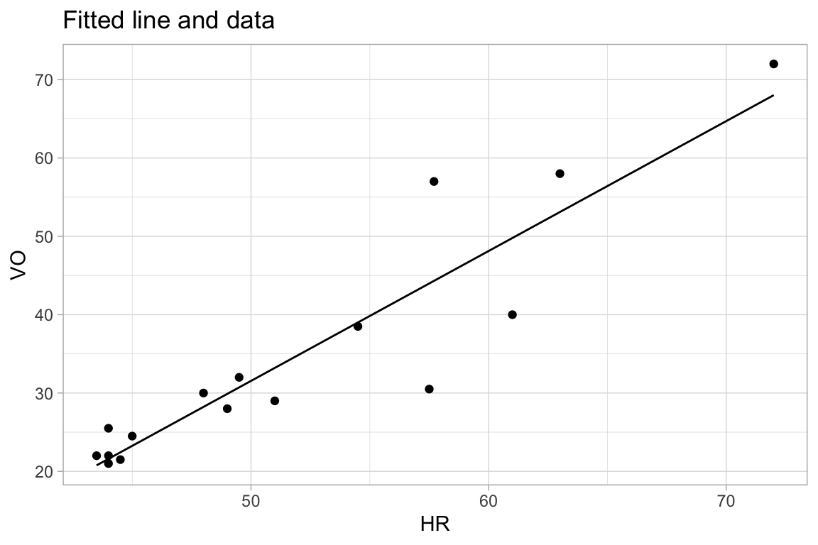

12:75 - Victoria Paukova

Code

df = tibble(
  x=c(10,8,13,9,11,14,6,4,12,7,5),
  y1=c(8.04,6.95,7.58,8.81,8.33,9.96,7.24,4.26,10.84,4.82,5.68),
  y2=c(9.14,8.14,8.74,8.77,9.26,8.1,6.13,3.1,9.13,7.26,4.74),
  y3=c(7.46,6.77,12.74,7.11,7.81,8.84,6.08,5.39,8.15,6.42,5.73),
  x4=c(8,8,8,8,8,8,8,19,8,8,8),
  y4=c(6.58,5.76,7.71,8.84,8.47,7.04,5.25,12.5,5.56,7.91,6.89))

12:75 - Victoria Paukova

Code

model1 = lm(y1 ~ x, data=df)
model2 = lm(y2 ~ x, data=df)
model3 = lm(y3 ~ x, data=df)
model4 = lm(y4 ~ x4, data=df)

summary(model1)
summary(model2)
summary(model3)
summary(model4)


Call:
lm(formula = y1 ~ x, data = df)

Residuals:
     Min       1Q   Median       3Q      Max 
-1.92127 -0.45577 -0.04136  0.70941  1.83882 

Coefficients:
            Estimate Std. Error t value Pr(>|t|)   
(Intercept)   3.0001     1.1247   2.667  0.02573 * 
x             0.5001     0.1179   4.241  0.00217 **
---
Signif. codes:  0 '***' 0.001 '**' 0.01 '*' 0.05 '.' 0.1 ' ' 1

Residual standard error: 1.237 on 9 degrees of freedom
Multiple R-squared:  0.6665,    Adjusted R-squared:  0.6295 
F-statistic: 17.99 on 1 and 9 DF,  p-value: 0.00217


Call:
lm(formula = y2 ~ x, data = df)

Residuals:
    Min      1Q  Median      3Q     Max 
-1.9009 -0.7609  0.1291  0.9491  1.2691 

Coefficients:
            Estimate Std. Error t value Pr(>|t|)   
(Intercept)    3.001      1.125   2.667  0.02576 * 
x              0.500      0.118   4.239  0.00218 **
---
Signif. codes:  0 '***' 0.001 '**' 0.01 '*' 0.05 '.' 0.1 ' ' 1

Residual standard error: 1.237 on 9 degrees of freedom
Multiple R-squared:  0.6662,    Adjusted R-squared:  0.6292 
F-statistic: 17.97 on 1 and 9 DF,  p-value: 0.002179


Call:
lm(formula = y3 ~ x, data = df)

Residuals:
    Min      1Q  Median      3Q     Max 
-1.1586 -0.6146 -0.2303  0.1540  3.2411 

Coefficients:
            Estimate Std. Error t value Pr(>|t|)   
(Intercept)   3.0025     1.1245   2.670  0.02562 * 
x             0.4997     0.1179   4.239  0.00218 **
---
Signif. codes:  0 '***' 0.001 '**' 0.01 '*' 0.05 '.' 0.1 ' ' 1

Residual standard error: 1.236 on 9 degrees of freedom
Multiple R-squared:  0.6663,    Adjusted R-squared:  0.6292 
F-statistic: 17.97 on 1 and 9 DF,  p-value: 0.002176


Call:
lm(formula = y4 ~ x4, data = df)

Residuals:
   Min     1Q Median     3Q    Max 
-1.751 -0.831  0.000  0.809  1.839 

Coefficients:
            Estimate Std. Error t value Pr(>|t|)   
(Intercept)   3.0017     1.1239   2.671  0.02559 * 
x4            0.4999     0.1178   4.243  0.00216 **
---
Signif. codes:  0 '***' 0.001 '**' 0.01 '*' 0.05 '.' 0.1 ' ' 1

Residual standard error: 1.236 on 9 degrees of freedom
Multiple R-squared:  0.6667,    Adjusted R-squared:  0.6297 
F-statistic:    18 on 1 and 9 DF,  p-value: 0.002165

12:75 - Victoria Paukova

Code

ggplot(df, aes(x,y1)) + 
  geom_point() + 
  geom_smooth(method="lm", se=FALSE) + 
  labs(title="Scatter Plot 1")
ggplot(df, aes(x,y2)) + 
  geom_point() + 
  geom_smooth(method="lm", se=FALSE) + 
  labs(title="Scatter Plot 2")
ggplot(df, aes(x,y3)) + 
  geom_point() + 
  geom_smooth(method="lm", se=FALSE) + 
  labs(title="Scatter Plot 3")
ggplot(df, aes(x4,y4)) + 
  geom_point() + 
  geom_smooth(method="lm", se=FALSE) + 
  labs(title="Scatter Plot 4")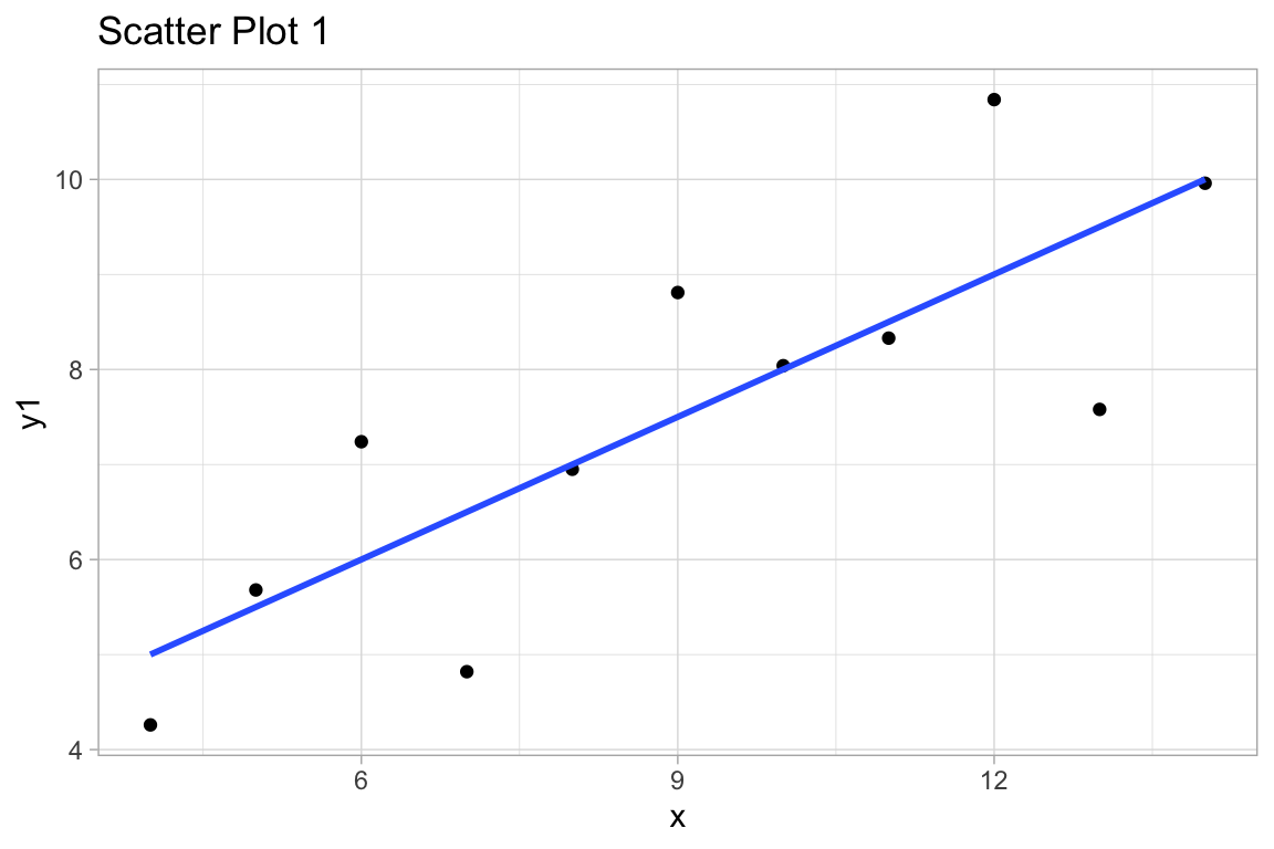

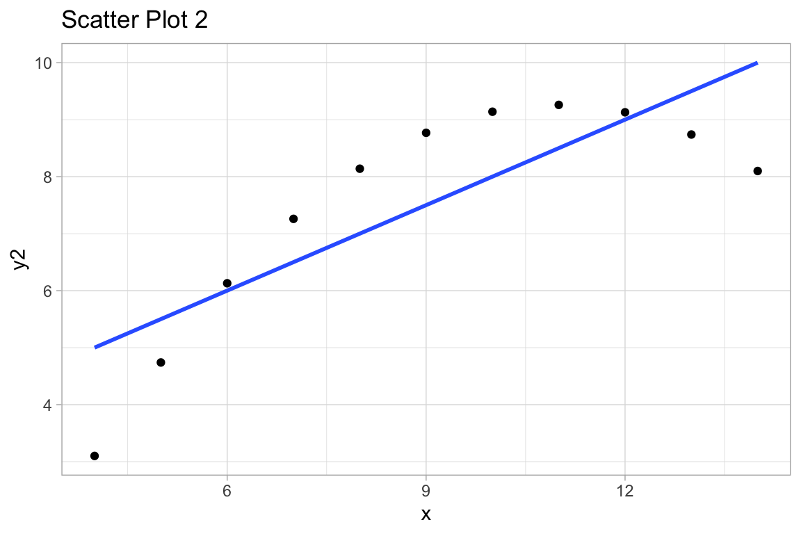
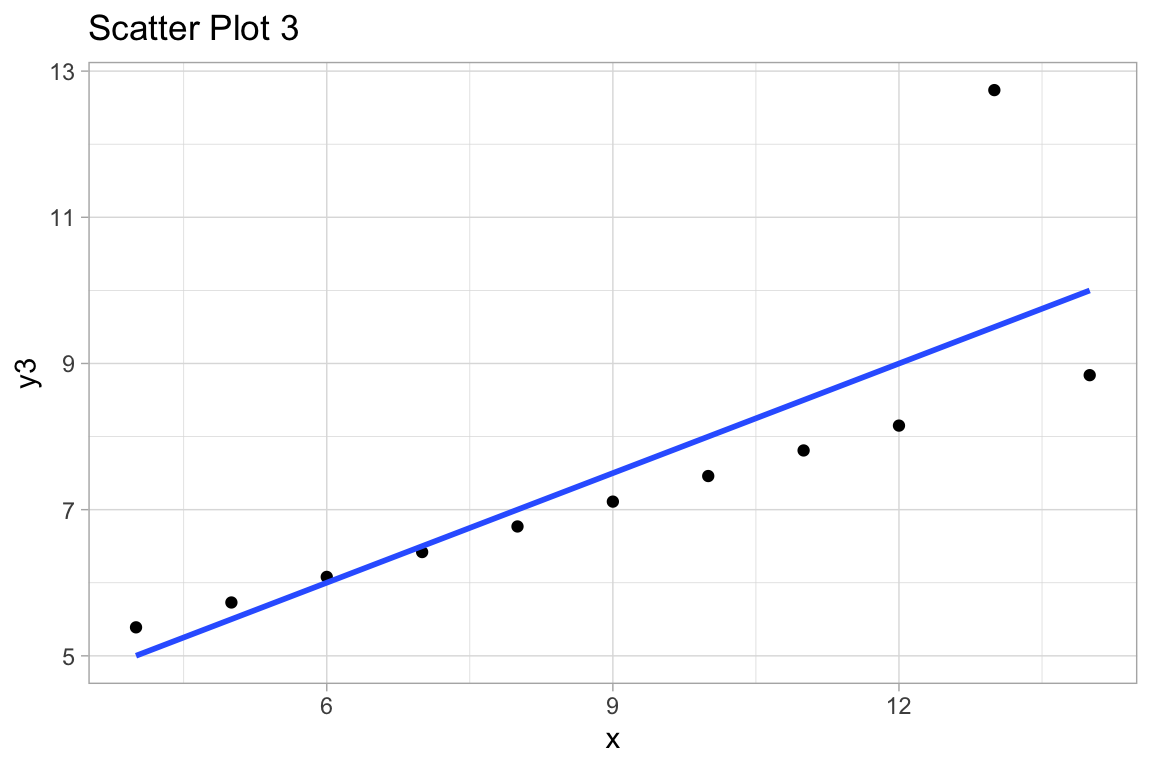
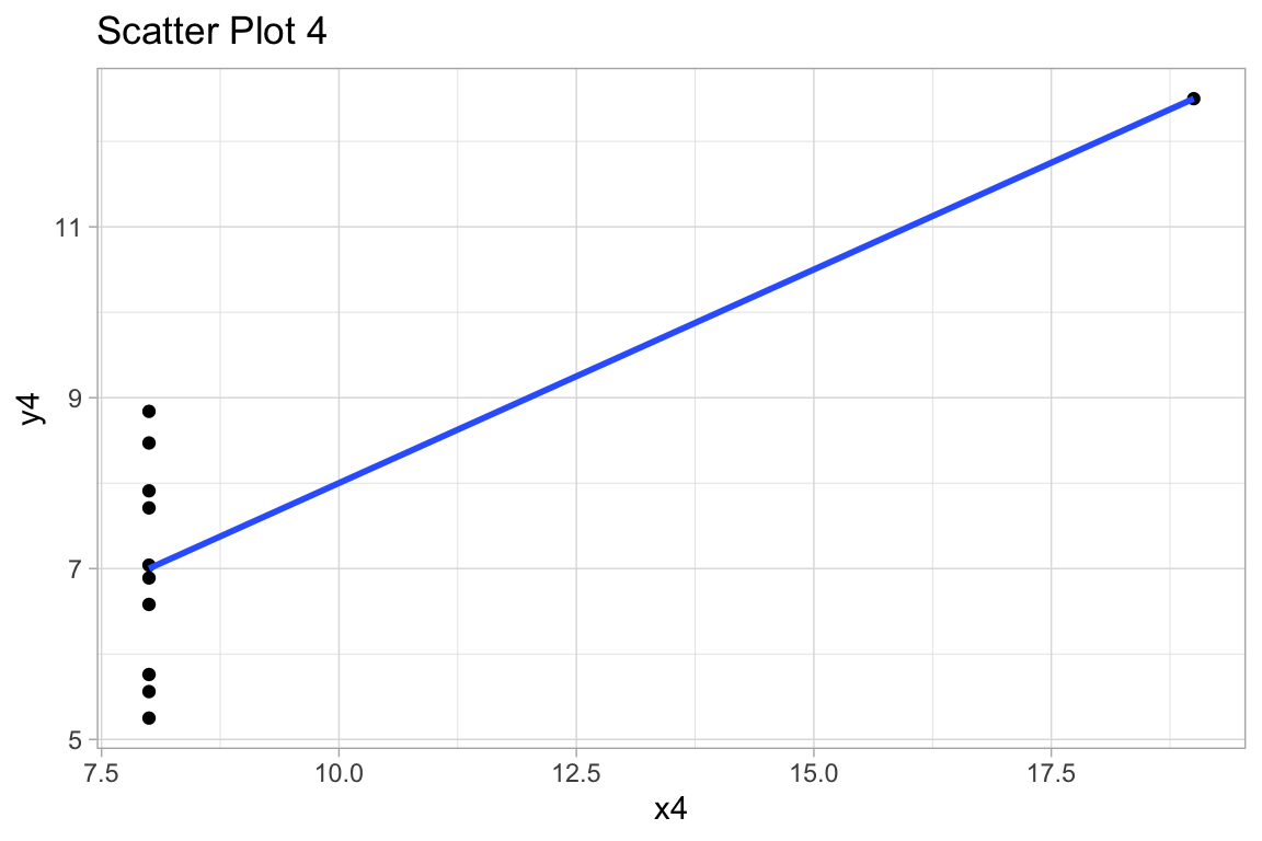
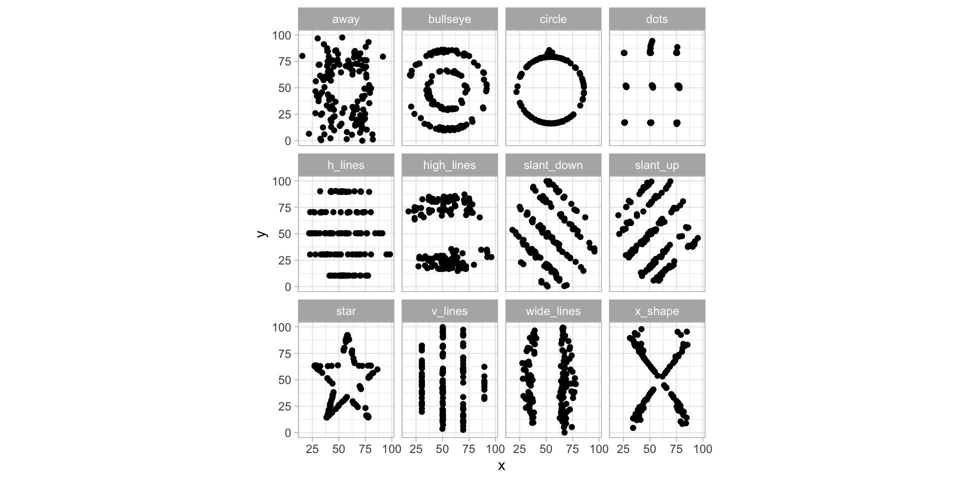
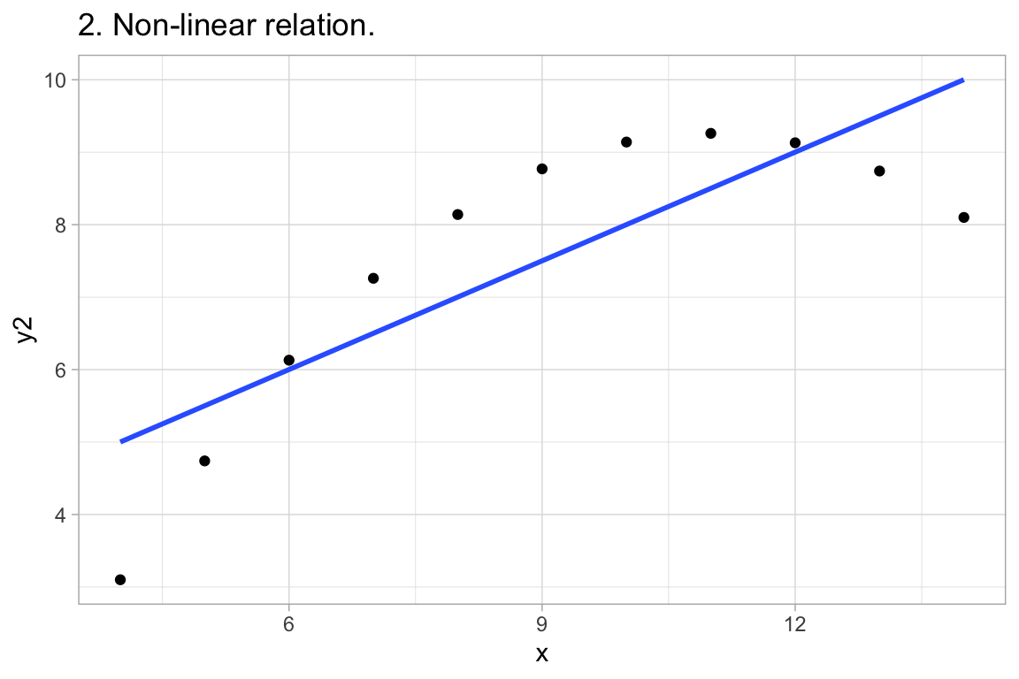
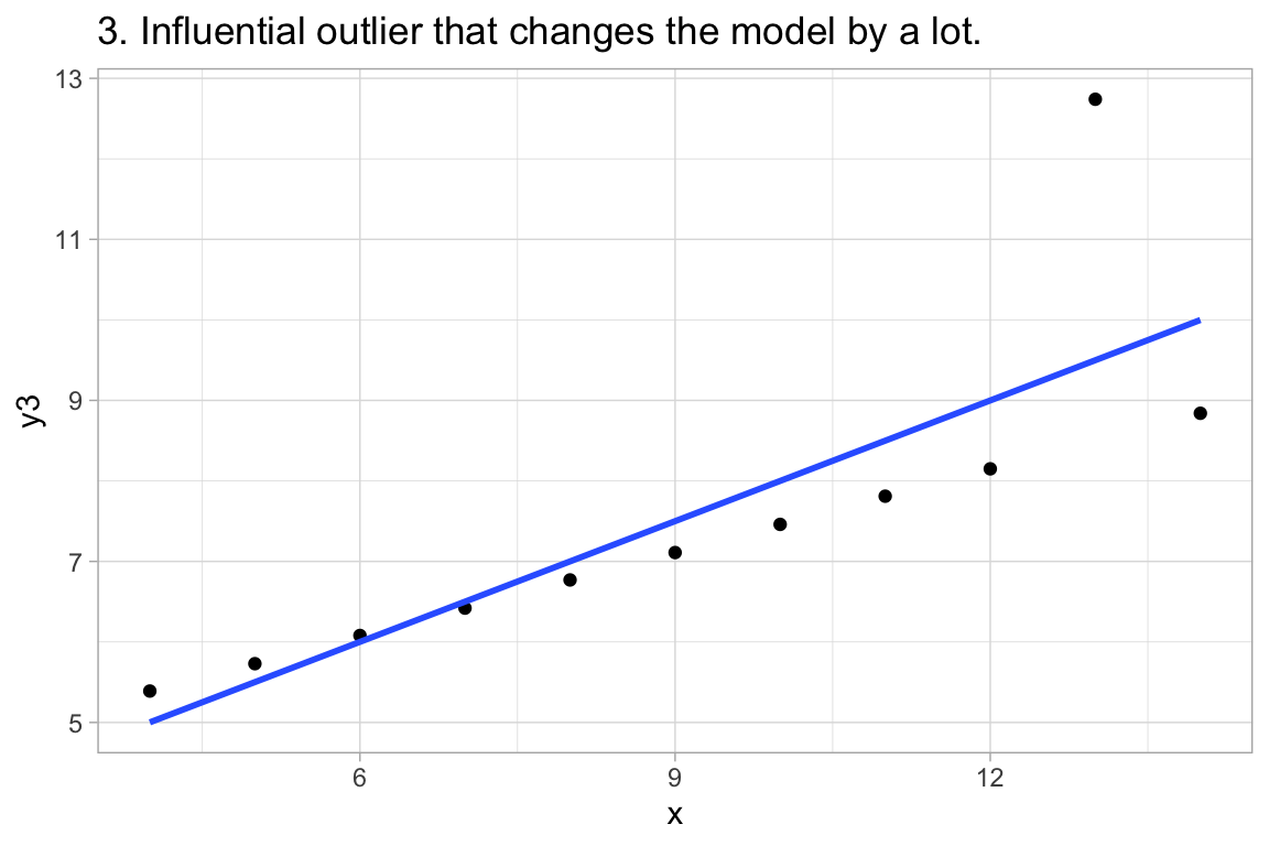
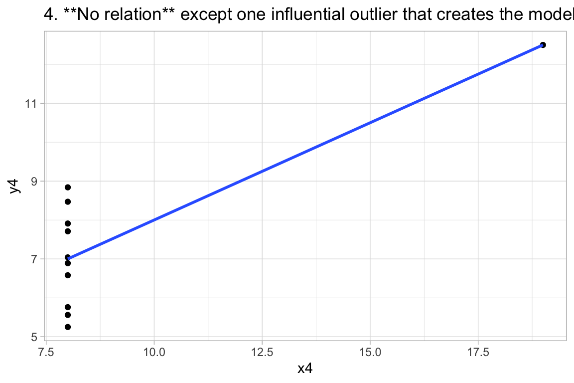
12:75 - Victoria Paukova

Code

library(ggfortify)

autoplot(list(model1,model2,model3,model4), which=1:3, ncol=3) #+ coord_fixed()

Anscombe’s Quartet

12:75 deals with Anscombe’s Quartet, an example of 4 paired datasets with:

Equal means in both variables ($x=9$, $y=7.5$)
Equal variance in both variables ($x=11$, $y=4.125$)
Equal correlations (0.816)
Equal linear models ($y=3+0.5x$)
Equal coefficients of determination (0.67)

Code

ggplot(df, aes(x,y1)) + 
  geom_point() + 
  geom_smooth(method="lm", se=FALSE) + 
  labs(title="1. Reasonable linear model application.")
ggplot(df, aes(x,y2)) + 
  geom_point() + 
  geom_smooth(method="lm", se=FALSE) + 
  labs(title="2. Non-linear relation.")
ggplot(df, aes(x,y3)) + 
  geom_point() + 
  geom_smooth(method="lm", se=FALSE) + 
  labs(title="3. Influential outlier that changes the model by a lot.")
ggplot(df, aes(x4,y4)) + 
  geom_point() + 
  geom_smooth(method="lm", se=FALSE) + 
  labs(title="4. **No relation** except one influential outlier that creates the model.")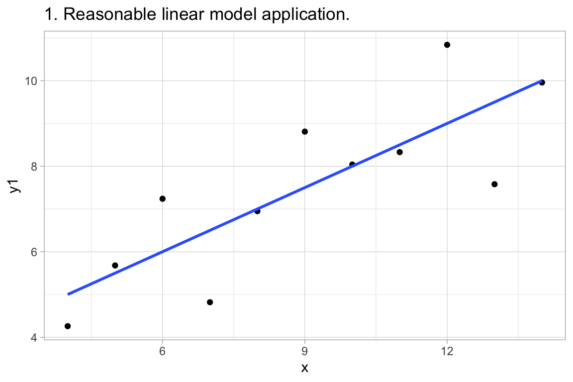

Datasaurus Dozen

Code

library(datasauRus)

ggplot(datasaurus_dozen %>% filter(dataset != "dino"), aes(x=x, y=y)) +
  geom_point() + 
  coord_fixed() +
  facet_wrap(~dataset)

Datasaurus Dozen

Code

datasaurus_dozen %>% 
  filter(dataset != "dino") %>%
  group_by(dataset) %>%
  summarise(mean.x = mean(x), mean.y = mean(y), sd.x = sd(x), sd.y = sd(y), 
            cor = cor(x,y), beta.1 = cor*sd.y/sd.x, 
            beta.0 = mean.y - beta.1*mean.x, sigma = sqrt((1-cor^2)*sd.y^2)) %>%
  kable(digits = 2)

dataset	mean.x	mean.y	sd.x	sd.y	cor	beta.1	beta.0	sigma
away	54.27	47.83	16.77	26.94	-0.06	-0.10	53.43	26.88
bullseye	54.27	47.83	16.77	26.94	-0.07	-0.11	53.81	26.87
circle	54.27	47.84	16.76	26.93	-0.07	-0.11	53.80	26.87
dots	54.26	47.84	16.77	26.93	-0.06	-0.10	53.10	26.88
h_lines	54.26	47.83	16.77	26.94	-0.06	-0.10	53.21	26.89
high_lines	54.27	47.84	16.77	26.94	-0.07	-0.11	53.81	26.88
slant_down	54.27	47.84	16.77	26.94	-0.07	-0.11	53.85	26.87
slant_up	54.27	47.83	16.77	26.94	-0.07	-0.11	53.81	26.88
star	54.27	47.84	16.77	26.93	-0.06	-0.10	53.33	26.88
v_lines	54.27	47.84	16.77	26.94	-0.07	-0.11	53.89	26.87
wide_lines	54.27	47.83	16.77	26.94	-0.07	-0.11	53.63	26.88
x_shape	54.26	47.84	16.77	26.93	-0.07	-0.11	53.55	26.87

Datasaurus Dozen

Code

ggplot(datasaurus_dozen %>% filter(dataset == "dino"), aes(x=x, y=y)) +
  geom_point() + 
  coord_fixed()


\(n=n_{,}=\sum_{i=1}^I\sum_{j=1}^J n_{i,j}\)	total number of observations
\(n_{i,j}\)	The count of occurrences of the \(j\)th category paired with the \(i\)th category
\(n_{*,j}=\sum_{i=1}^I n_{ij}\)	the count of occurrences of the \(j\)th category
\(n_{i,*}=\sum_{j=1}^Jn_{i,j}\)	the count of occurrences of the \(i\)th category
\(p_{i,j}=n_{i,j}/n_{,}\)	overall proportion of observation in the \(i,j\) cell
\(p_{j\|i}=n_{i,j}/n_{i,*}\)	proportion of observations with the \(i\)th category that fall into category \(j\).
\(p_{i,}=n_{i,}/n_{,}\)	proportion of occurrences of category \(i\) in the entire dataset
\(p_{,j}=n_{,j}/n_{,}\)	proportion of occurrences of category \(j\) in the entire population

	MM	MF	FF
1	0.0	0.1	0.4
2	0.1	0.7	1.0
3	0.1	0.4	0.3
4	0.3	0.5	0.3
5	0.0	0.1	0.2
6	0.4	0.1	1.5

	MM	MF	FF
1	0.0	0.1	0.4
2	0.1	0.7	1.0
3	0.1	0.4	0.3
4	0.3	0.5	0.3
5	0.0	0.1	0.2
6	0.4	0.1	1.5

	MM	MF	FF
1	0.0	0.1	0.4
2	0.1	0.7	1.0
3	0.1	0.4	0.3
4	0.3	0.5	0.3
5	0.0	0.1	0.2
6	0.4	0.1	1.5