
Linear Regression
Mikael Vejdemo-Johansson
\[ \def\RR{{\mathbb{R}}} \def\PP{{\mathbb{P}}} \def\EE{{\mathbb{E}}} \def\VV{{\mathbb{V}}} \]
What if my model is not normal?
Logistic, Poisson and Generalized Linear Models
A Generalized Linear Model consists of
- An exponential family probability distribution for modeling \(Y\)
- A linear predictor \(\eta = X\beta\) (matrix-vector multiplication)
- A link function \(g\) such that \(\EE[Y|X] = g^{-1}(\eta)\)
The model is fitted using maximum likelihood with iterative updates
What if my model is not normal?
Logistic, Poisson and Generalized Linear Models
| Distribution | Link | Link Function | Mean Function | |
|---|---|---|---|---|
| Normal | Identity | \(X\beta = \mu\) | \(\mu = X\beta\) | |
| Bernoulli | Logit | \(X\beta = \log\left(\frac{\mu}{1-\mu}\right)\) | \(\mu = \frac{\exp[X\beta]}{1+\exp[X\beta]}=\frac{1}{1+\exp[-X\beta]}\) | |
| Binomial | Logit | \(X\beta = \log\left(\frac{\mu}{1-\mu}\right)\) | \(\mu = \frac{\exp[X\beta]}{1+\exp[X\beta]}=\frac{1}{1+\exp[-X\beta]}\) | |
| Poisson | Log | \(X\beta = \log(\mu)\) | \(\mu=\exp[X\beta]\) | |
| Exponential | Negative Inverse | \(X\beta = -1/\mu\) | \(\mu = -1/(X\beta)\) |
Logistic Regression
Logistic Regression is the specific choice of using the logit function as a link function in a GLM for predicting probabilities.
This function continuously re-maps \(\RR\) to \([0,1]\), mapping \(0\mapsto 0.5\) and with horizontal asymptotes at 0 and 1.
Many components of this setup map to interpretable quantities:
Odds: The odds at some predictor value \(y=\beta_0+\beta_1x\) is \[ o(y)=\frac{p(y)}{1-p(y)}= \frac{\frac{\exp[y]}{1+\exp[y]}}{1-\frac{\exp[y]}{1+\exp[y]}} = \frac{\frac{\exp[y]}{1+\exp[y]}}{\frac{1+\exp[y]}{1+\exp[y]}-\frac{\exp[y]}{1+\exp[y]}} = \frac{\frac{\exp[y]}{1+\exp[y]}}{\frac{1}{1+\exp[y]}} = \exp[y] \]
Odds Ratio: For a unit increase in the predictor, the odds ratio is given by: \[ OR = \frac{o(x+1)}{o(x)} = \frac{\exp[\beta_0+\beta_1(x+1)]}{\exp[\beta_0+\beta_1x]} = \exp[\beta_1] \]
GLM in software
GLM is implemented in statsmodels.api.GLM. You choose which type to run using the objects in statsmodels.api.families.*:
import statsmodels.api as sms
import numpy as np

x = [0.50,0.75,1.00,1.25,1.50,1.75,1.75,2.00,2.25,2.50,
     2.75,3.00,3.25,3.50,4.00,4.25,4.50,4.75,5.00,5.50]
y = [0,0,0,0,0,0,1,0,1,0,
     1,0,1,0,1,1,1,1,1,1]

glm = sms.GLM(y, sms.tools.add_constant(x), family=sms.families.Binomial())
results = glm.fit()
results.params # offset, slope
results.pvalues # for the offset and slope
results.predict([1,3.75]) # include the 1 for the intercept constant
GLM is handled by the function glm. You pick type by providing a family function (such as gaussian, binomial, poisson, …):
df = tibble(
  x = c(0.50,0.75,1.00,1.25,1.50,1.75,1.75,2.00,2.25,2.50,
        2.75,3.00,3.25,3.50,4.00,4.25,4.50,4.75,5.00,5.50),
  y = c(0,0,0,0,0,0,1,0,1,0,
        1,0,1,0,1,1,1,1,1,1)
)

model = glm(y~x, family=binomial(), data=df)

model
anova(model)
summary(model)
model$coefficients
predict(model, tibble(x=3.75), type="response")
Logistic Regression Example
Exercise 12.44
A study on the relationship between amount of job experience and the likelihood of success at a certain complex task collected the following data:
Code
df = rbind(tibble(success = c(8, 13, 14, 18, 20, 21, 21, 22, 25, 26, 28, 29, 30, 32), failure=NA),
  tibble(failure = c(4, 5, 6, 6, 7, 9, 10, 11, 11, 13, 15, 18, 19, 20, 23, 27), success=NA)) %>%
  mutate(id=row_number()) %>%
  pivot_longer(-id, values_drop_na=TRUE, names_to="outcome", values_to="months") %>%
  mutate(outcome=as.integer(outcome=="success"))

df[1:15,] %>% t %>% kable| id | 1 | 2 | 3 | 4 | 5 | 6 | 7 | 8 | 9 | 10 | 11 | 12 | 13 | 14 | 15 |
| outcome | 1 | 1 | 1 | 1 | 1 | 1 | 1 | 1 | 1 | 1 | 1 | 1 | 1 | 1 | 0 |
| months | 8 | 13 | 14 | 18 | 20 | 21 | 21 | 22 | 25 | 26 | 28 | 29 | 30 | 32 | 4 |
| id | 16 | 17 | 18 | 19 | 20 | 21 | 22 | 23 | 24 | 25 | 26 | 27 | 28 | 29 | 30 |
| outcome | 0 | 0 | 0 | 0 | 0 | 0 | 0 | 0 | 0 | 0 | 0 | 0 | 0 | 0 | 0 |
| months | 5 | 6 | 6 | 7 | 9 | 10 | 11 | 11 | 13 | 15 | 18 | 19 | 20 | 23 | 27 |
Logistic Regression Example
Exercise 12.44
We fit a logistic regression to the given data:
Call:
glm(formula = outcome ~ months, family = binomial(), data = df)

Deviance Residuals:
    Min       1Q   Median       3Q      Max
-1.8833  -0.7079  -0.4148   0.8527   1.9717

Coefficients:
            Estimate Std. Error z value Pr(>|z|)
(Intercept) -3.21107    1.23540  -2.599  0.00934 **
months       0.17772    0.06573   2.704  0.00686 **
---
Signif. codes:  0 '***' 0.001 '**' 0.01 '*' 0.05 '.' 0.1 ' ' 1

(Dispersion parameter for binomial family taken to be 1)

    Null deviance: 41.455  on 29  degrees of freedom
Residual deviance: 30.799  on 28  degrees of freedom
AIC: 34.799

Number of Fisher Scoring iterations: 4 2.5 % 97.5 %
(Intercept) -6.08783298 -1.0870563
months 0.06439767 0.3298068 1 2 3 4
0.1048213 0.2537965 0.4969589 0.7415684 Poisson Regression Example
Data was collected on how many high school students were diagnosed with a particular infectious disease by the number of days past the onset of an outbreak at the school.
Code
cases = tibble(
  days=c(1, 2, 3, 3, 4, 4, 4, 6, 7, 8,
8, 8, 8, 12, 14, 15, 17, 17, 17, 18, 19, 19, 20,
23, 23, 23, 24, 24, 25, 26, 27, 28, 29, 34, 36, 36,
42, 42, 43, 43, 44, 44, 44, 44, 45, 46, 48, 48, 49,
49, 53, 53, 53, 54, 55, 56, 56, 58, 60, 63, 65, 67,
67, 68, 71, 71, 72, 72, 72, 73, 74, 74, 74, 75, 75,
80, 81, 81, 81, 81, 88, 88, 90, 93, 93, 94, 95, 95,
95, 96, 96, 97, 98, 100, 101, 102, 103, 104, 105,
106, 107, 108, 109, 110, 111, 112, 113, 114, 115),
  students=c(6, 8, 12, 9, 3, 3, 11, 5, 7, 3, 8,
    4, 6, 8, 3, 6, 3, 2, 2, 6, 3, 7, 7, 2, 2, 8,
    3, 6, 5, 7, 6, 4, 4, 3, 3, 5, 3, 3, 3, 5, 3,
    5, 6, 3, 3, 3, 3, 2, 3, 1, 3, 3, 5, 4, 4, 3,
    5, 4, 3, 5, 3, 4, 2, 3, 3, 1, 3, 2, 5, 4, 3,
    0, 3, 3, 4, 0, 3, 3, 4, 0, 2, 2, 1, 1, 2, 0,
    2, 1, 1, 0, 0, 1, 1, 2, 2, 1, 1, 1, 1, 0, 0,
    0, 1, 1, 0, 0, 0, 0, 0)
)
Poisson Regression Example
Call:
glm(formula = students ~ days, family = poisson(), data = cases)

Deviance Residuals:
     Min        1Q    Median        3Q       Max
-2.00482  -0.85719  -0.09331   0.63969   1.73696

Coefficients:
             Estimate Std. Error z value Pr(>|z|)
(Intercept)  1.990235   0.083935   23.71   <2e-16 ***
days        -0.017463   0.001727  -10.11   <2e-16 ***
---
Signif. codes:  0 '***' 0.001 '**' 0.01 '*' 0.05 '.' 0.1 ' ' 1

(Dispersion parameter for poisson family taken to be 1)

    Null deviance: 215.36  on 108  degrees of freedom
Residual deviance: 101.17  on 107  degrees of freedom
AIC: 393.11

Number of Fisher Scoring iterations: 5
Poisson Regression Example
Inference & prediction for specific \(x^*\)
Pick a specific value \(x^*\) for the predictor variable \(x\). Once \(\hat\beta_0\) and \(\hat\beta_1\) have been estimated, both a point estimate of \(\EE[Y(x^*)]\) and a point prediction of \(Y(x^*)\) are given by \(\hat\beta_0+\hat\beta_1x^*\).
Difference between these two cases is not in the point estimate, but in the degree of uncertainty.
Note: \[ \begin{align*} \color{Teal}{\hat\beta_0}+\color{DarkMagenta}{\hat\beta_1}x^* &= \color{Teal}{\overline Y-\hat\beta_1\overline x} + \color{DarkMagenta}{\hat\beta_1}x^* = \overline Y + \hat\beta_1(x^*-\overline x) = \overline Y+\frac{S_{xy}}{S_{xx}}(x^*-\overline x) \\ &= \overline Y+\frac{\sum_i(x_i-\overline x)(Y_i-\overline Y)}{S_{xx}}(x^*-\overline x) \\ &= \overline Y + \sum_i \frac{(x_i-\overline x)(x^*-\overline x)}{S_{xx}}Y_i - \overline Y\frac{(x^*-\overline x)}{S_{xx}}\underbrace{\sum_i(x_i-\overline x)}_{=0} \end{align*} \]
Inference & prediction for specific \(x^*\)
We arrive at: \[ \begin{align*} \hat\beta_0+\hat\beta_1x^* &= \overline Y + \sum_i \frac{(x_i-\overline x)(x^*-\overline x)}{S_{xx}}Y_i \\ &= \sum_i\left({1\over n} + {(x_i-\overline x)(x^*-\overline x)\over S_{xx}}\right)Y_i \end{align*} \]
So with coefficients \(d_i={1\over n}+{(x_i-\overline x)(x^*-\overline x)\over S_{xx}}\), the prediction is a linear combination of independent normal variables, and therefore has a normal sampling distribution.
\(\hat\beta_0+\hat\beta_1x^*\) is unbiased
We check the expected value \[ \EE[\hat\beta_0+\hat\beta_1x^*] = \EE[\hat\beta_0]+\EE[\hat\beta_1]x^* = \beta_0+\beta_1x^* \]
Standard Error of \(\hat\beta_0+\hat\beta_1x^*\)
Exercise 12.55
\[ \begin{align*} \VV[\hat\beta_0+\hat\beta_1x^*] &= \VV\left[\sum_i d_i Y_i\right] = \sum_i d_i^2\VV[Y_i] \\ &= \sum_i\left({1\over n}+{(x_i-\overline x)(x^*-\overline x)\over S_{xx}}\right)^2\color{Teal}{\VV\left[Y_i\right]} \\ &= \color{Teal}{\sigma^2}\left( n{1\over n^2} + 2{(x^*-\overline x)\over n S_{xx}}\underbrace{\sum_i(x_i-\overline x)}_{=0} + {(x^*-\overline x)^2 \over S_{xx}}\underbrace{\sum_i(x_i-\overline x)^2 \over S_{xx}}_{=1} \right) \\ &= \sigma^2\left({1 \over n} + {(x^*-\overline x)^2 \over S_{xx}}\right) \end{align*} \]
T-distribution and pivot
Theorem
\[ T = {(\hat\beta_0+\hat\beta_1x^*) - (\beta_0+\beta_1x^*) \over S_{\hat\beta_0+\hat\beta_1x^*}} = {\hat Y(x^*) - Y(x^*)\over S_{\hat Y(x^*)}} \sim T(n-2) \]
Proof
Under our assumptions, \[ {\hat Y(x^*)-Y(x^*) \over \sigma\sqrt{{1\over n}+{(x^*-\overline x)^2 \over S_{xx}}}} \sim \mathcal{N}(0,1) \qquad\text{and}\qquad {(n-2)S^2\over \sigma^2}\sim\chi^2(n-2) \]
Replacing \(\sigma\) with \(S\) proceeds the same way as all our previous \(T\)-distribution proofs.
Hypothesis Test and Confidence Intervals
Hypothesis Test for Linear Regression Means
- Null Hypothesis
- \(\hat Y(x^*) = Y_0\)
- Test Statistic
- \(t = {\hat Y(x^*) - Y_0 \over S\sqrt{{1\over n}+{(x^*-\overline x)^2 \over S_{xx}}}}\)
| Alternative Hypothesis | Rejection Region for Level \(\alpha\) | p-value | |
|---|---|---|---|
| Upper Tail | \(t>t_{\alpha,n-2}\) | \(1-CDF_{T(n-2)}(t)\) | |
| Two-tailed | \(|t|>t_{\alpha/2,n-2}\) | \(2\min\{CDF_{T(n-2)}(t), 1-CDF_{T(n-2)}(t)\}\) | |
| Lower Tail | \(t<-t_{\alpha,n-2}\) | \(CDF_{T(n-2)}(t)\) |
- \(1-\alpha\) Confidence Interval
- \(Y(x^*) \in \hat Y(x^*)\pm t_{\alpha/2, n-2}S\sqrt{{1\over n}+{(x^*-\overline x)^2 \over S_{xx}}}\)
Prediction Interval
In order to predict the value \(Y(x^*)\), we need to study not the estimation error \((\beta_0+\beta_1x^*)-(\hat\beta_0+\hat\beta_1x^*)\) but the prediction error \(Y(x^*)-(\hat\beta_0+\hat\beta_1x^*) = (\beta_0+\beta_1x^*+\epsilon)-(\hat\beta_0+\hat\beta_1x^*)\).
The prediction is unbiased, but the variance is different: \[ \begin{align*} \VV[Y(x^*)-(\hat\beta_0+\hat\beta_1x^*)] &= \VV[Y(x^*)] + \VV[\hat\beta_0+\hat\beta_1x^*] \\ &= \VV[\epsilon] + \sigma^2\left({1\over n}+{(x^*-\overline x)^2 \over S_{xx}}\right) \\ &= \sigma^2\left(1+{1\over n}+{(x^*-\overline x)^2 \over S_{xx}}\right) \end{align*} \]
From the same T-distribution argument as above, we get a prediction interval:
\[ Y(x^*) \in \hat\beta_0+\hat\beta_1x^*\pm t_{\alpha/2,n-2}S\sqrt{1+{1\over n}+{(x^*-\overline x)^2 \over S_{xx}}} \]
Covariance
For the joint distribution of two random variables \(X\) and \(Y\), their covariance measures the extent to which they tend to vary the same way: \[ Cov(X,Y) = \EE[(X-\EE[X])(Y-\EE[Y])] \]
A very large covariance means that whenever \(X\) is larger than \(\EE[X]\), it tends to be accompanied with a \(Y\) larger than \(\EE[Y]\).
A covariance near 0 means that \(X\) and \(Y\) are nearly independent of each other.
A covariance that is very large, but negative, means that whenever \(X\) is larger than \(\EE[X]\), it tends to be accompanied with a \(Y\) much smaller (or more negative) than \(\EE[Y]\).
Covariance
Code
covar_df = tibble(
  x = rnorm(25),
  y = x,
  y1 = y + rnorm(25, sd=0.25),
  y2 = y + rnorm(25, sd=2.5),
  y3 = rnorm(25, sd(y)),
  y4 = -y + rnorm(25, sd=2.5),
  y5 = -y + rnorm(25, sd=0.25)
) %>% pivot_longer(starts_with("y")) %>% filter(name != "y")

ggplot(covar_df, aes(x,value)) +
  geom_point() +
  facet_grid(~name) +
  coord_fixed(xlim=c(-3,3), ylim=c(-5,5))
covar_df %>%
  group_by(name) %>%
  summarise(cov(x, value)) %>%
  t %>%
  kable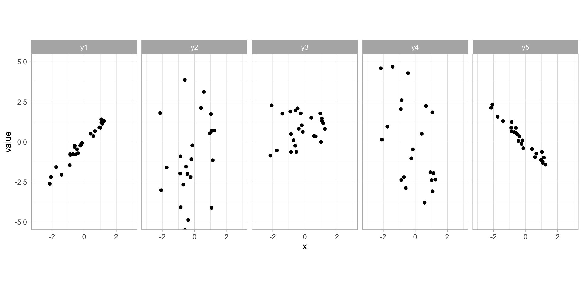
| name | y1 | y2 | y3 | y4 | y5 |
| cov(x, value) | 1.1244711 | 1.1811299 | 0.1651461 | -1.3684579 | -1.0697642 |
Covariance
Why was \(Cov(x,y_2)\) and \(Cov(x,y_4)\) so much bigger than \(Cov(x,y_1)\) and \(Cov(x,y_5)\)?
Wasn’t covariance supposed to be bigger if the variables vary similar to each other?
Covariance is very sensitive to scale: \[ Cov(\lambda X, Y) = \EE[(\lambda X - \EE[\lambda X])(Y-\EE[Y])] = \EE[\lambda(X-\EE[X])(Y-\EE[Y])] = \lambda Cov(X,Y) \]
So by just changing our measurement units for one variable, we can achieve any degree of large or small covariance we want!
Code
| name | y1 | y2 | y3 | y4 | y5 |
| cov | 1.1244711 | 1.1811299 | 0.1651461 | -1.3684579 | -1.0697642 |
| sd(y) | 1.1299523 | 3.0991859 | 0.9560964 | 3.4661892 | 1.0751270 |
| cov(x,y/sd(y)) | 0.9951492 | 0.3811097 | 0.1727295 | -0.3948018 | -0.9950120 |
Correlation
There is no intrinsic reason to believe \(Y\) needs to change and \(X\) does not. So we might as well normalize both:
Definition
The correlation of two random variables \(X\) and \(Y\) with means \(\mu_X,\mu_Y\) and standard deviations \(\sigma_X,\sigma_Y\) is: \[ \rho(X,Y) = \EE\left[ \left({X-\mu_X\over\sigma_X}\right)\cdot \left({Y-\mu_Y\over\sigma_Y}\right) \right] \]
Definition
The sample correlation of two paired sets of observations \((x_1,y_1),\dots,(x_n,y_n)\) is \[ r(x,y) = \frac{1}{n-1}\sum \left({x_i-\overline x\over s_x}\right)\cdot \left({y_i-\overline y\over s_y}\right) = {S_{xy}\over\sqrt{S_{xx}}\sqrt{S_{yy}}} \]
This specific sample correlation is sometimes called Pearson Correlation or Pearson’s \(\rho\). There are others (Spearman’s \(\rho\), Kendall’s \(\tau\)) in wide use for other situations.
Properties of sample correlation
Theorem
- \(r(x,y) = r(y,x)\) (does not depend on labels)
- \(r(x,y) = r(\lambda x,y)\) (does not depend on measurement units)
- \(-1 \leq r(x,y) \leq 1\)
- \(r(x,y)\in\{-1,1\}\) iff all \((x_i,y_i)\) pairs lie on a straight line - \(1\) if that line has positive slope, \(-1\) if the line has negative slope.
- \(r^2\) is the coefficient of determination (ie fraction of explained variance) that would result from fitting a linear regression to the data.
Proof
- is immediate from the symmetries of the definition.
Properties of sample correlation
Theorem
- \(r(x,y) = r(\lambda x,y)\) (does not depend on measurement units)
- \(-1 \leq r(x,y) \leq 1\)
- \(r(x,y)\in\{-1,1\}\) iff all \((x_i,y_i)\) pairs lie on a straight line - \(1\) if that line has positive slope, \(-1\) if the line has negative slope.
- \(r^2\) is the coefficient of determination (ie fraction of explained variance) that would result from fitting a linear regression to the data.
Proof
For 2., note that if \(u_i=ax_i+b\) then \(\overline u={a\sum x_i+nb\over n}=a\overline x+b\), and \(s_u^2 = \sum {(ax_i+b-a\overline x-b)^2\over n-1} = a^2\sum{(x_i-\overline x)^2\over n-1} = a^2s_x^2\). Similarly for \(v_i=cy_i+d\). Then consider: \[ \begin{align*} r(ax+b, cy+d) &= \sum \left(u_i-\overline u\over s_u\right)\cdot \left(v_i-\overline v\over s_v\right) \\ &= \sum \left(ax_i+\color{Teal}{b} - a\overline x\color{Teal}{-b} \over as_x\right)\cdot \left(cy_i+\color{DarkMagenta}{d} - c\overline y\color{DarkMagenta}{-d} \over cs_y\right) \\ &= \sum \left(\color{Teal}{a}\sum x_i-\overline x\over \color{Teal}{a}s_x\right)\cdot \left(\color{DarkMagenta}{c}\sum y_i-\overline y\over\color{DarkMagenta}{c}s_y\right) = r(x,y) \end{align*} \]
Properties of sample correlation
Theorem
- \(-1 \leq r(x,y) \leq 1\)
- \(r(x,y)\in\{-1,1\}\) iff all \((x_i,y_i)\) pairs lie on a straight line - \(1\) if that line has positive slope, \(-1\) if the line has negative slope.
- \(r^2\) is the coefficient of determination (ie fraction of explained variance) that would result from fitting a linear regression to the data.
Proof
For 5., recall the anova equation for regression: \(SST = SSE+SSR = SSE+\sum(\hat y_i-\overline y)^2\). We saw last lecture that \(\hat y_i-\overline y = \hat\beta_1(x_i-\overline x)\), and it follows that
\[ \begin{align*} \sum (\hat y_i-\overline y)^2 &= \hat\beta_1^2\sum(x_i-\overline x)^2 = \left(S_{xy}\over S_{xx}\right)^2S_{xx} \\ &= {(S_{xy})^2\over (S_{xx})^2}S_{xx}\cdot {S_{yy}\over S_{yy}} = {(S_{xy})^2\over S_{xx}S_{yy}}\cdot S_{yy} = r^2\cdot SST \end{align*} \]
So \(SST = SSE + r^2\cdot SST\), and it follows \(r^2={SST-SSE\over SST}\), which proves property 5. Since \(SSE\leq SST\), property 3. follows directly.
Properties of sample correlation
Theorem
- \(r(x,y)\in\{-1,1\}\) iff all \((x_i,y_i)\) pairs lie on a straight line - \(1\) if that line has positive slope, \(-1\) if the line has negative slope.
Proof
Finally, the only case in which \(SSE=0\) (and therefore \(r^2=SST/SST=1\) and \(r=\pm 1\)) is when all the points are actually on the regression line, which proves property 4.
What does \(r\) measure?
Since it is so tightly connected (through properties 4 and 5) to linear regression, Pearson’s \(r\) measures the degree of linear relationship between variables.
When should I care?
Different research fields can have vastly different conventions as to what is a weak or strong correlation. Our book suggests weak to mean \(0\leq|r|\leq0.5\) and strong to mean \(0.8\leq|r|\leq 1\), but this is far from universal.
\(r\) as point estimate
\(r\) is a point estimate for \(\rho\), observed from an estimator \[ \hat\rho = R = {\sum(X_i-\overline X)(Y_i-\overline Y) \over \sqrt{\sum(X_i-\overline X)^2}\sqrt{\sum(Y_i-\overline Y)^2}} \]
Bivariate Normal Distribution
Suppose \(\boldsymbol\Sigma\) is a positive definite symmetric matrix, and \[ \begin{pmatrix} X_i \\ Y_i \end{pmatrix} \sim\mathcal{N}\left( \begin{pmatrix} \mu_X \\ \mu_Y \end{pmatrix}, \begin{pmatrix} \Sigma_{XX} & \Sigma_{XY} \\ \Sigma_{YX} & \Sigma_{YY} \end{pmatrix} \right) = \mathcal{N}(\boldsymbol\mu, \boldsymbol\Sigma) \\ \text{with density } PDF(\boldsymbol{x}) = {1\over\sqrt{(2\pi)^2\det(\boldsymbol\Sigma)}} \exp\left[ -{1\over2}(\boldsymbol{x}-\boldsymbol\mu)^T\boldsymbol\Sigma^{-1}(\boldsymbol{x}-\boldsymbol\mu) \right] \]
We can identify \(\begin{pmatrix}\Sigma_{XX} & \Sigma_{XY} \\ \Sigma_{YX} & \Sigma_{YY}\end{pmatrix}=\begin{pmatrix}\sigma_X^2 & \rho\sigma_X\sigma_Y \\ \rho\sigma_X\sigma_Y & \sigma_Y^2\end{pmatrix}\) (the covariance matrix of the distribution), and by doing this we can unpack the density function \[ PDF\left(\begin{pmatrix}x \\ y\end{pmatrix}\right) = {1\over2\pi\sigma_X\sigma_Y\sqrt{1-\rho^2}} \exp\left[ -\left[ \left(x-\mu_X \over \sigma_X\right)^2 -2\rho{(x-\mu_X)\over\sigma_X}{(y-\mu_Y)\over\sigma_Y} +\left(y-\mu_Y\over\sigma_Y\right)^2 \over 2(1-\rho^2) \right] \right] \]
This distribution has marginal densities \[ PDF_{Y|X=x}(y) = \mathcal{N}\left(\mu_Y+\rho\sigma_Y{x-\mu_X\over\sigma_X}, \sigma_Y^2(1-\rho^2)\right) \]
Linear Regression on Bivariate Normal data
\[ PDF_{Y|X=x}(y) = \mathcal{N}\left(\mu_Y+\rho{\sigma_Y\over\sigma_X}(x-\mu_X), \sigma_Y^2(1-\rho^2)\right) = \\ \mathcal{N}\left(\color{Teal}{\underbrace{\mu_Y-\rho{\sigma_Y\over\sigma_X}\mu_X}_{=\beta_0}}+\color{DarkMagenta}{\underbrace{\rho{\sigma_Y\over\sigma_X}}_{=\beta_1}}x, \color{DarkGoldenrod}{\underbrace{\sigma_Y^2(1-\rho^2)}_{=\sigma^2}}\right) \]
For bivariate normal data, the simple linear regression as we have described it is the appropriate probabilistic model.
Hypothesis Test for \(\rho=0\)
Exercise 65
Theorem
When \(H_0:\rho=0\) is true, the test statistic \[ T = {R\sqrt{n-2}\over\sqrt{1-R^2}}\sim T(n-2) \]
Proof
We unpack the ratio, using \(\hat\beta_1=r{\sigma_Y\over\sigma_X}\) and that \(r^2=1-SSE/SST\): \[ \begin{align*} T = {R\sqrt{n-2}\over\sqrt{1-R^2}} &= {\hat\beta_1{\sigma_X\over\sigma_Y}\sqrt{n-2} \over\sqrt{SSE/SST}} = {\hat\beta_1{\color{DarkMagenta}{\sqrt{S_{XX}}}\over\color{DarkGoldenrod}{\sqrt{S_{YY}}}}\color{DarkGoldenrod}{\sqrt{SST}} \over \color{Teal}{\sqrt{SSE/(n-2)}}} \\ &={\hat\beta_1\over\color{Teal}{S}/\color{DarkMagenta}{\sqrt{S_{XX}}}} \end{align*} \]
…which is the \(T\) ratio used for testing \(H_0:\beta_1=0\), and we already know that this \(T\) ratio is distributed as \(T(n-2)\).
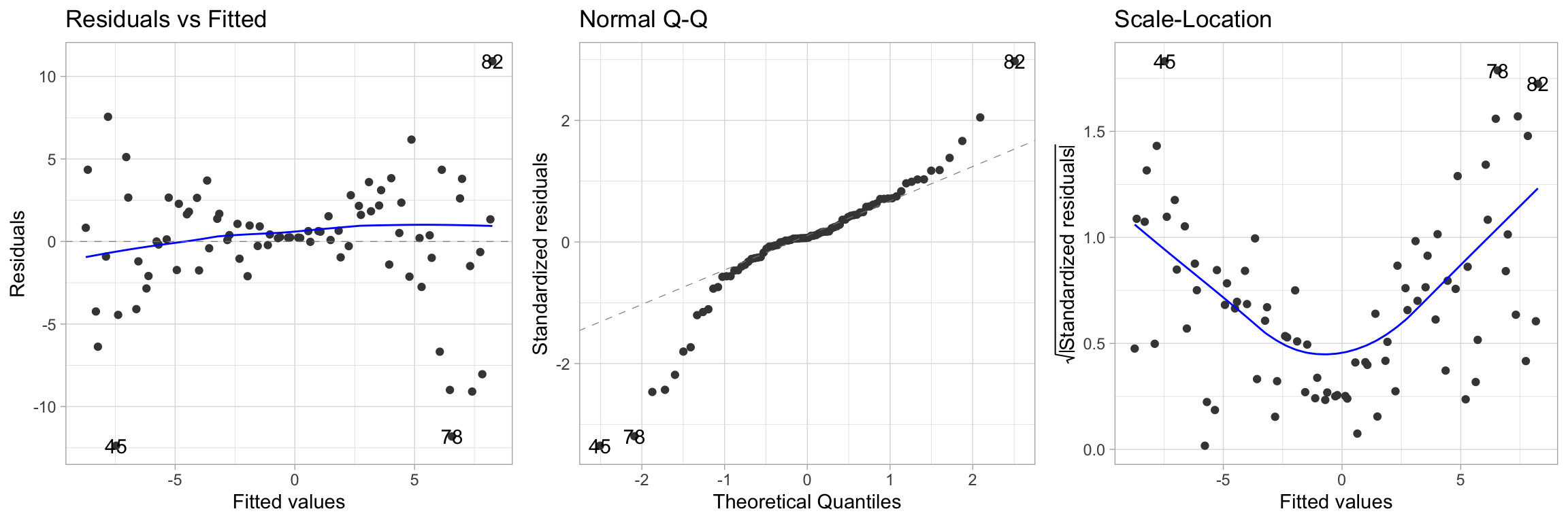
Model Diagnostics
There are 5 fundamentally important plots for evaluating whether a linear regression is a good fit to a particular data set:
- Scatter plot \(y_i\) vs. \(x_i\) (this does not generalize well to multivariate)
- Scatter plot \(y_i\) vs. \(\hat y_i\)
- Scatter plot \(e_i\) vs. \(x_i\) (this does not generalize well to multivariate)
- Scatter plot \(e_i\) vs. \(\hat y_i\)
- Normal probability plot of \(e_i\)
Model Diagnostics
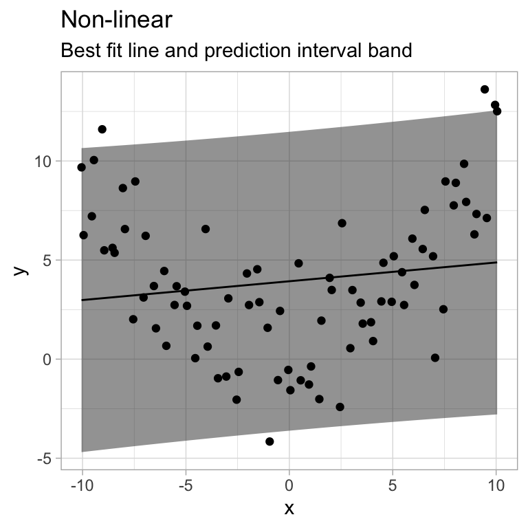
There are 6 commonly occurring problems with linear regressions:
- The relationship between \(x\) and \(y\) is better modeled with a non-linear function. (maybe you need different predictors?)
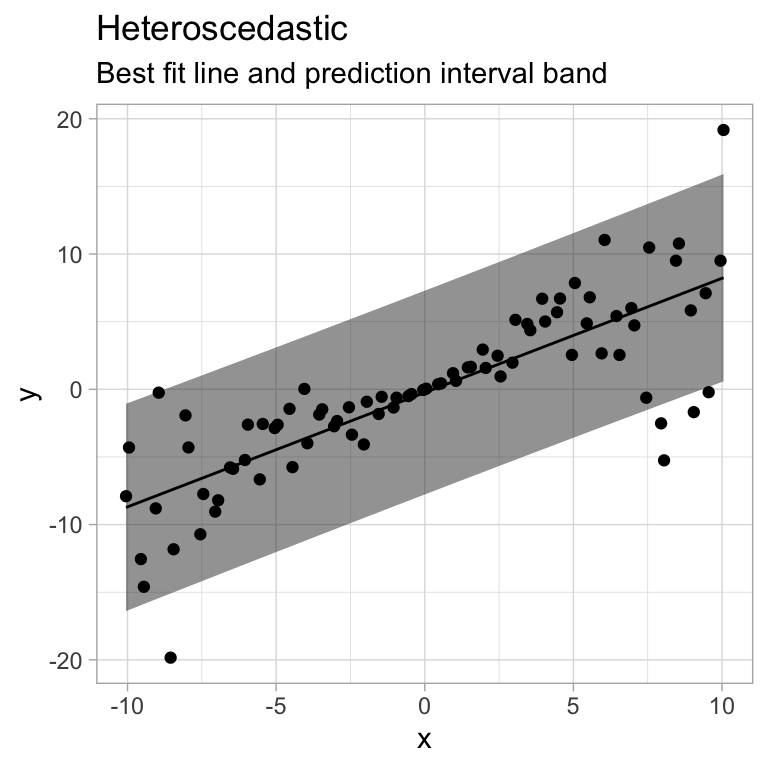
- The variance varies with \(x\) (heteroscedasticity)
- The model fits well except for a few outliers that influence the model by a lot
- The residuals are not normally distributed
- The residuals are not independent of each other
- One or more relevant variables have been omitted
Model Diagnostics
Code
diag_df = tibble(
  x=rep(seq(-10,10,by=0.5),2)+c(-0.05,0.05),
  t=abs(x+runif(length(x),-0.1,0.1)),
  yl=x+rnorm(length(x), sd=2.5),
  yq=0.1*(x-mean(x))^2+mean(x)^2+rnorm(length(x),sd=2.5),
  yhs=x+rnorm(length(x), sd=t^1.5*0.25)
)
diag_df_long = diag_df %>%
  pivot_longer(starts_with("y")) %>%
  mutate(name=fct_recode(name, heteroscedastic="yhs", linear="yl", `non-linear`="yq"))

ggplot(diag_df_long, aes(x,value)) +
  geom_point() +
  facet_grid(~name) +
  labs(title="Different failure modes",y="y")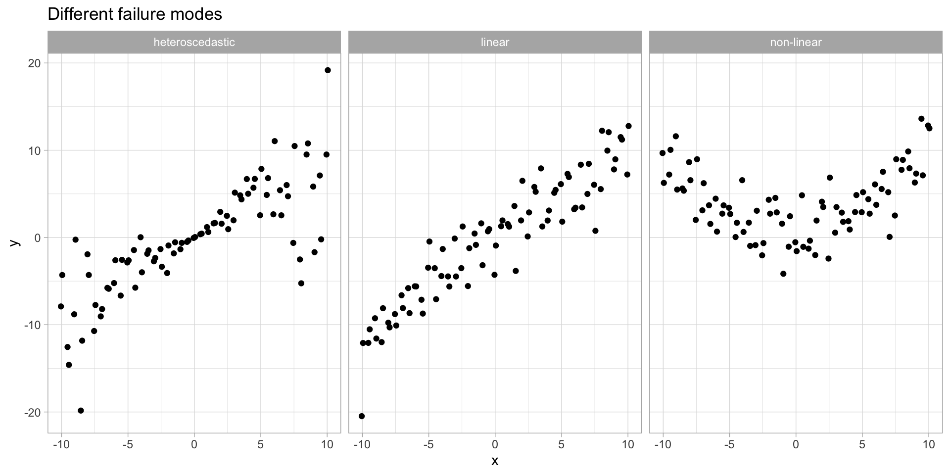
Model Diagnostics - Data 1
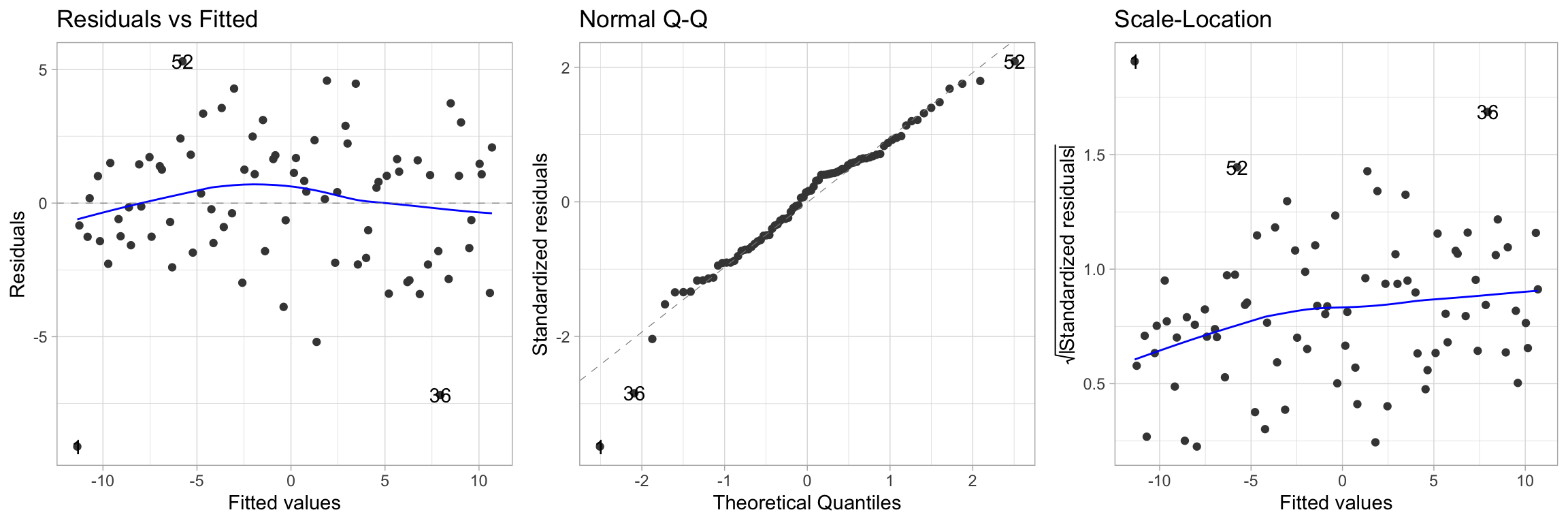
Model Diagnostics - Data 2
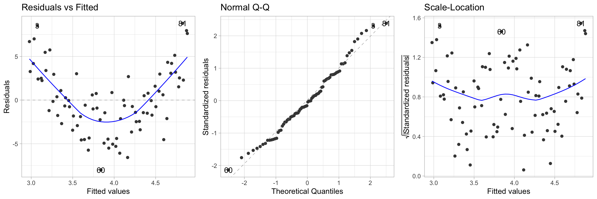
Model Diagnostics - Data 3
Model Fits
Code
library(broom)

plot.model = function(model, yvar, name) {
  ggplot(augment(model, diag_df, interval="prediction")) +
    geom_ribbon(aes(x,{{yvar}},ymin=.lower,ymax=.upper), alpha=0.5) +
    geom_point(aes(x,{{yvar}})) +
    geom_line(aes(x,.fitted)) +
    labs(title=name, subtitle="Best fit line and prediction interval band", x="x", y="y")
}

plot.model(model1, yl, "Linear")
plot.model(model2, yq, "Non-linear")
plot.model(model3, yhs, "Heteroscedastic")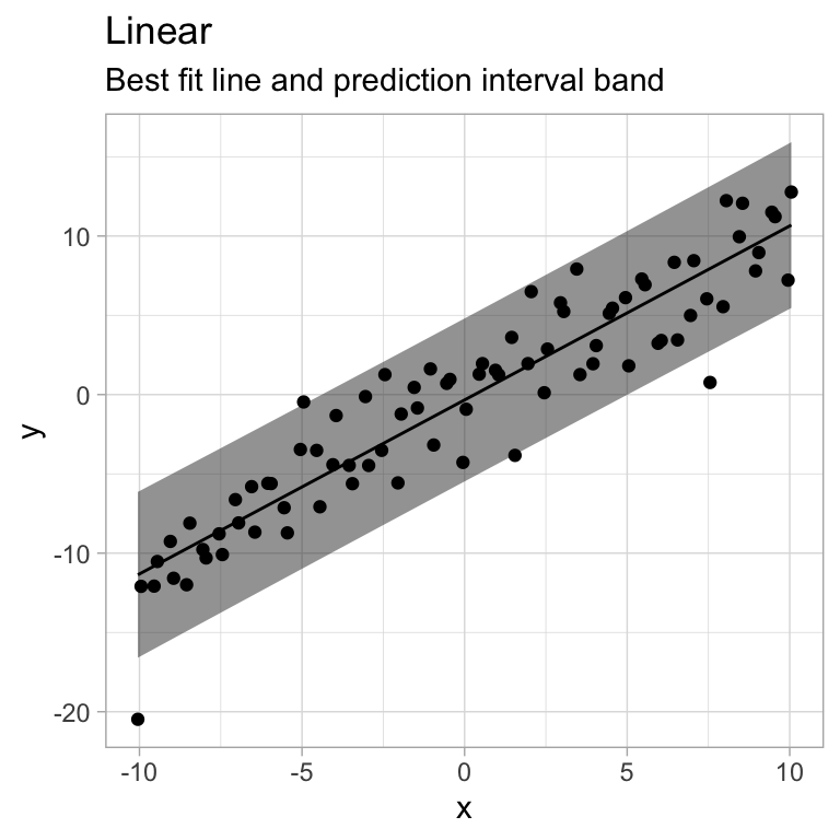
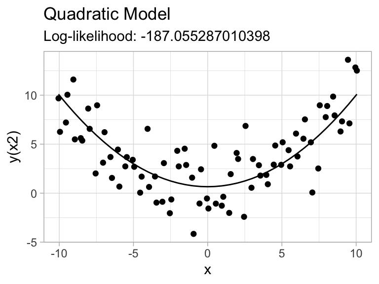
Model Selection
If we have several candidate models, we can consider choosing based on something like a maximum likelihood argument.
The linear regression function in R, lm, will give you a computed log-likelihood of the fitted parameters given the data. We could, for instance, try predicting with \(x^2\) as predictor instead of \(x\):
Code
ggplot(augment(model_linear, diag_df)) +
  geom_point(aes(x,yq)) +
  geom_line(aes(x,.fitted)) +
  labs(x="x",y="y(x)", title="Linear Model",
       subtitle=str_glue("Log-likelihood: {glance(model_linear)$logLik}"))
ggplot(augment(model_quadratic, diag_df)) +
  geom_point(aes(x,yq)) +
  geom_line(aes(x,.fitted)) +
  labs(x="x",y="y(x2)", title="Quadratic Model",
       subtitle=str_glue("Log-likelihood: {glance(model_quadratic)$logLik}"))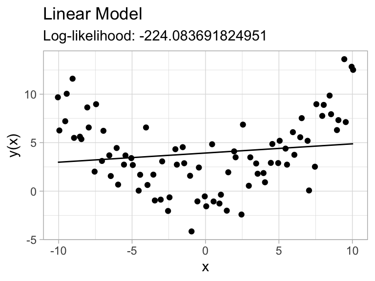
Your Homework
11.8 - Maxim Kleyer
Code
wheat = np.array([5.2, 4.5, 6.0, 6.1, 6.7, 5.8])
barley = np.array([6.5, 8.0, 6.1, 7.5, 5.9, 5.6])
maize = np.array([5.8, 4.7, 6.4, 4.9, 6.0, 5.2])
oats = np.array([8.3, 6.1, 7.8, 7.0, 5.5, 7.2])

# Normal probability plot
pyplot.figure(figsize=(8, 6))

ax = pyplot.subplot(2, 2, 1)
p = scipy.stats.probplot(wheat, plot=ax)
ax.set_title('Wheat: Normal Probability Plot')

ax = pyplot.subplot(2, 2, 2)
p = scipy.stats.probplot(barley, plot=ax)
ax.set_title('Barley: Normal Probability Plot')

ax = pyplot.subplot(2, 2, 3)
p = scipy.stats.probplot(maize, plot=ax)
ax.set_title('Maize: Normal Probability Plot')

ax = pyplot.subplot(2, 2, 4)
p = scipy.stats.probplot(oats, plot=ax)
ax.set_title('Oats: Normal Probability Plot')

pyplot.show()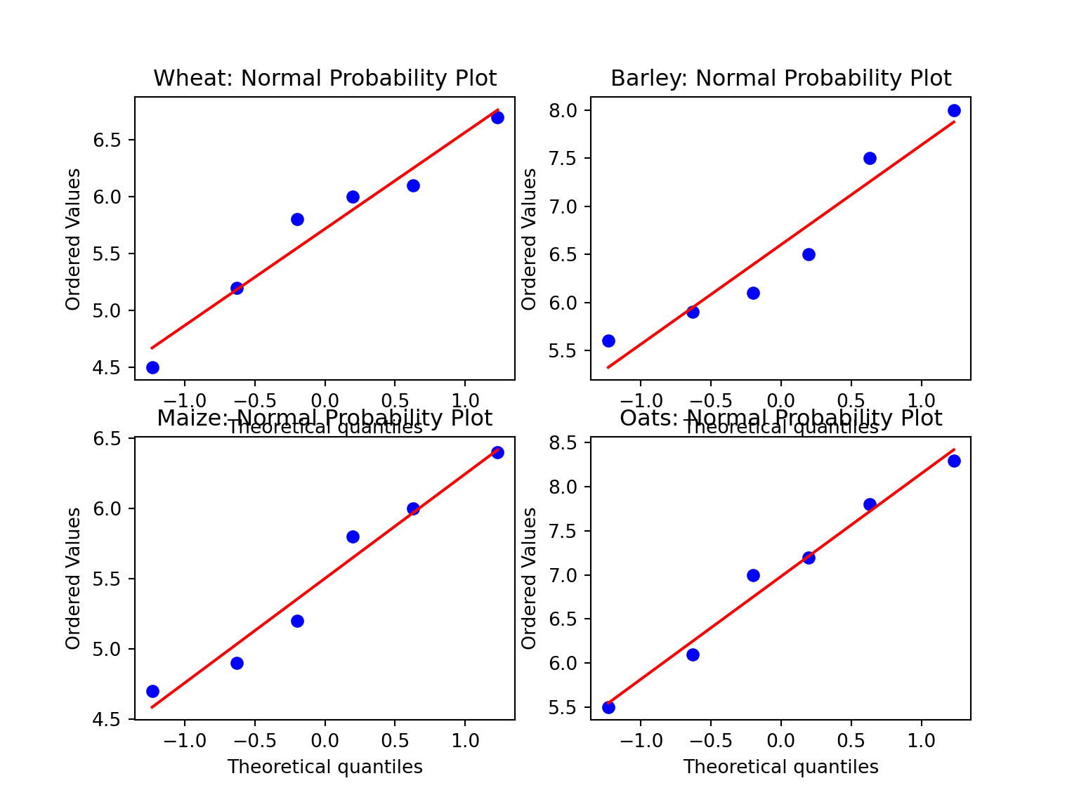
11.8 - Maxim Kleyer
Code
Levene's Test for Equal Variances:
Test Statistic: 0.31178
p-value: 0.81663
Code
One-Way ANOVA:
F-statistic: 3.95654
p-value: 0.02293
There is significant evidence to reject the null hypothesis.
11.10 a. - Nicholas Basile
\(\mu = {1\over I}\sum \mu_i\)
a.: Given: \(\overline X = {1\over I}\sum\overline X_i\) \[ \begin{align*} \EE[\overline X] &= \EE\left[{1\over I}\sum\overline X_i\right] \\ &= {1\over I}\sum\underbrace{\EE[\overline X_i]}_{=\mu_i} \\ &= {1\over I}\sum \mu_i \\ &= \mu \end{align*} \]
11.10 b. - Nicholas Basile
b.:
\[ \begin{align*} \EE[\overline X_i^2] &= \VV[\overline X_i] + \EE[\overline X_i]^2 \\ &= \VV\left[\sum_j X_{ij}\over J\right]+\mu_i^2 \\ &= {\sigma^2\over J}+\mu_i^2 \end{align*} \]
11.10 c. - Nicholas Basile
c.:
\[ \begin{align*} \EE[\overline X^2] &= \VV[\overline X] + \EE[\overline X]^2 \\ &= \VV\left[\sum\overline X_{ij}\over IJ\right] + \mu^2 \\ &= {\sigma^2\over IJ}+\mu^2 \end{align*} \]
11.10 d. - Maxim Kleyer
d.:
\[ \begin{align*} \EE[SSTr] &= \EE\left[\sum_i J_iX_i^2-nX_{*,*}^2\right] \\ &= \sum_i J_i\EE[X_i^2]-n\EE[X_{*,*}^2] \\ &= \sum_i J_i\left[\VV[X_i]+\EE[X_i]^2\right]-n\left[\VV[X_{*,*}]+\EE[X_{*,*}]^2\right] \\ &= \sum_i J_i\left[{\sigma^2\over J_i}+\mu_i^2\right]-n\left[{\sigma^2\over n}+\overline\mu^2\right] \\ &= I\sigma^2+\sum_i J_i\mu_i^2 - \sigma^2 - n\overline\mu^2 \\ &= (I-1)\sigma^2 + J\sum(\mu_i^2-2\mu_i\mu+\mu^2) \\ &= \EE[MSTr]\cdot(I-1) \end{align*} \]
11.10 e. - Maxim Kleyer
e.: \(H_0:\mu_i=\mu\) - when \(H_0\) is true, \(MSTr\) is unbiased.
\(\EE[MSTr] = \sigma^2\)
\(H_a:(\mu_i-\mu)^2 > 0\)
\(\EE[MSTr] = \sigma^2+{J\over I-1}\sum_i(\mu_i-\mu)^2 > \sigma^2\)
11.11 - Justin Ramirez
a.:
The number of brands of yellow interior latex paint is \(I=5\)
Number of gallons in each paint are \(J=4\)
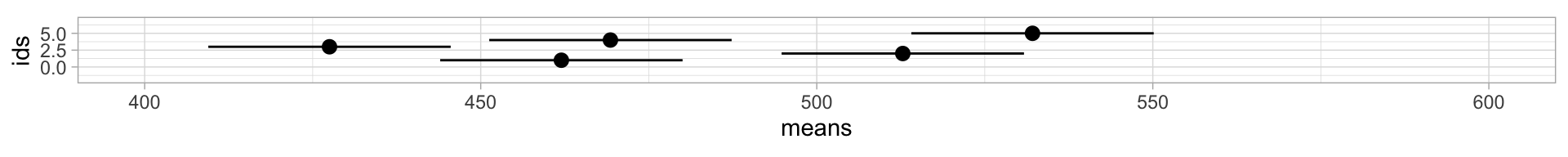
Sample means are: \[ \begin{align*} \overline x_1 &= 462.0 & \overline x_2 &= 512.8 & \overline x_3 &= 437.5 & \overline x_4 &= 469.3 & \overline x_5 &= 532.1 \end{align*} \]
The MSE is: \(272.8\)
The studentized range distribution (critical value) is \(Q_{\alpha,I,I(J-1)}=Q_{0.05,5,15}\approx 4.37\)
\[ \begin{align*} q &= Q\cdot\sqrt{MSE\over J} \Rightarrow 4.37\cdot\sqrt{272.8\over 4}\approx 36.09 \end{align*} \]
\[ \begin{align*} x_3 &= 437.5 & x_1 &= 462.0 & x_4 &= 469.3 & x_2 &= 512.8 & x_5 &= 532.1 \end{align*} \]
The tukey test asks to calculate the difference in means:
The differences in means that are less than \(w\): \[ \begin{align*} \overline x_1-\overline x_3 &= 24.5 & \overline x_4-\overline x_3 &= 31.8 & \overline x_4-\overline x_1 &= 7.3 & \overline x_5-\overline x_2 &= 19.3 \end{align*} \]
There is no significant difference between the brands of means \(\overline x_3, \overline x_1, \overline x_4\) and \(\overline x_2,\overline x_5\) within the groups, but there is significant difference of means between the groups.
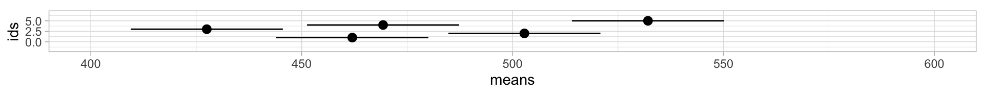
11.12 - Justin Ramirez
Referencing question 11.11 above
\[ \begin{align*} x_3 &= \color{Teal}{427.5} & x_1 &= 462.0 & x_4 &= 469.3 & x_2 &= 512.8 & x_5 &= 532.1 \end{align*} \]
With the changes to the value of \(\overline x_3\), brands 2 and 5 are not significantly different from each other, but are significantly higher than the other 3. While brand 4 is significantly better than brand 3 and brand 1 and 3 do not differ significantly.
11.13 - Justin Ramirez
In reference to the previous two questions
\[ \begin{align*} x_3 &= \color{Teal}{427.5} & x_1 &= 462.0 & x_4 &= 469.3 & x_2 &= \color{Teal}{502.8} & x_5 &= 532.1 \end{align*} \]
Using Tukey’s procedure, it can be concluded the \(\overline x_2\) and \(\overline x_5\) still do not differe significantly, while \(\overline x_2\) still differs significantly from \(\overline x_1\) and \(\overline x_3\). It does not significantly differ from \(\overline x_4\) as the difference is less than \(w\) which is 36.09.
11.11-13 Illustrated (MVJ)
Code
paint = tibble(
  ids=1:5,
  means=c(462.0,512.8,437.5,469.3,532.1)
)
MSE = 272.8
Q = qtukey(0.95, NROW(paint), 3*NROW(paint))
J = 4
w = Q*sqrt(MSE/J)

plotit = function(df) {
  df$means_lo = df$means-w/2
  df$means_hi = df$means+w/2

  ggplot(df, aes(x=means,y=ids,xmin=means_lo,xmax=means_hi)) +
    geom_pointrange() +
    coord_fixed(xlim=c(400,600), ylim=c(-2,7))
}

plotit(paint)
plotit(paint %>% mutate(means=replace(means, ids==3, 427.5)))
plotit(paint %>% mutate(means=replace(means, ids==3, 427.5)) %>% mutate(means=replace(means, ids==2, 502.8)))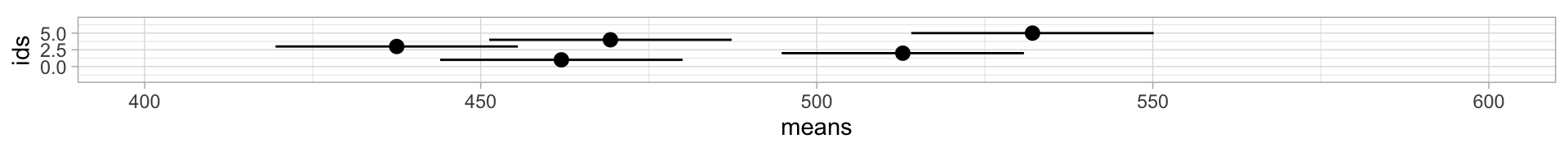
11.26 a. - Maxim Kleyer
a.: \(F=79.26\), \(p=1.7e-12 < .001\), we reject \(H_0\).
Can conclude at least one mean is different from others.
11.26 b. - Nicholas Basile
b.: \[ \begin{align*} (\overline x_i-\overline x_j)&\pm Q_{\alpha,I,I(J-1)}\cdot\sqrt{{MSE\over 2}\left({1\over J_i}+{1\over J_j}\right)} \\ Q_{.05,6,20} &\approx 4.445 \\ MSE &\approx .273 \end{align*} \]
Small Java-program included to run through all pairs. Here is a translation to Python:
Code
means = [14.1,12.8,13.825,13.1,17.14,18.1]
js = [4,5,4,4,5,4]

for i in range(6):
  for j in range(i+1,6):
    mdiff = means[i]-means[j]
    margin = 4.445*np.sqrt(.273/2*(1/js[i]+1/js[j]))
    sign = " "
    if np.abs(mdiff) > margin: sign="*"
    print(f"x{i+1} - x{j+1} in [{mdiff-margin:.3f}, {mdiff+margin:.3f}]{sign}")
x1 - x2 in [0.198, 2.402]*
x1 - x3 in [-0.886, 1.436]
x1 - x4 in [-0.161, 2.161]
x1 - x5 in [-4.142, -1.938]*
x1 - x6 in [-5.161, -2.839]*
x2 - x3 in [-2.127, 0.077]
x2 - x4 in [-1.402, 0.802]
x2 - x5 in [-5.379, -3.301]*
x2 - x6 in [-6.402, -4.198]*
x3 - x4 in [-0.436, 1.886]
x3 - x5 in [-4.417, -2.213]*
x3 - x6 in [-5.436, -3.114]*
x4 - x5 in [-5.142, -2.938]*
x4 - x6 in [-6.161, -3.839]*
x5 - x6 in [-2.062, 0.142] 11.26 c. - Nicholas Basile
c.: From 11.5: \(\sum c_i\overline x_i\pm t_{\alpha/2,I(J-1)}\sqrt{MSE\cdot\sum{c_i^2\over J}}\)
\(\hat\theta={14.1+12.8+13.825+13.1\over 4}-{17.14+18.1\over 2}\approx -4.16\)
\(\sum{c_i^2\over J_i}=\left(1\over 4\right)^2\left(\frac14+\frac15+\frac14+\frac14\right)+\left(-\frac12\right)^2\left(\frac15+\frac14\right)\approx .1719\)
\[ \begin{align*} \sum c_i\overline x_i&\pm t_{\alpha/2,I(J-1)}\sqrt{MSE\cdot\sum_i{c_i^2\over J_i }}\\ =-4.16&\pm 2.086\sqrt{.273\cdot.1719} =(-4.612,-3.708) \end{align*} \]
MVJ: I think the DoF for the T-distribution should be \(n-I\)? That’s what yields the critical value you use.