Linear Regression

Mikael Vejdemo-Johansson

\[ \def\RR{{\mathbb{R}}} \def\PP{{\mathbb{P}}} \def\EE{{\mathbb{E}}} \def\VV{{\mathbb{V}}} \]

Statistical Models

We have worked with one mean (one-sample T-tests), two means (two-sample T-tests), or several distinct means (ANOVA).

Now it is time to introduce the notion of predictors and models that depend on predictor variables.

We can see the cases we have already studied as specific cases where the predictors are variables that take on finitely many values:

One Mean

Predictor is (trivially and usually ignored) a constant value.

Two Means

Predictor takes two distinct values.

ANOVA

Predictor takes \(I\) distinct values.

Statistical Models

Definition

Given some set of predictor variables (aka independent v., explanatory v., covariate v., exposure v., manipulated v., input v., control v., exogenous v., regressor, risk factor, feature) \(X_1,\dots,X_n\) and some probabilistic model for error \(\epsilon\sim\mathcal{D}(X_1,\dots,X_n)\), an additive model specifies the values of some response variables (aka dependent v., explained v., predicted v., measured v., experimental v., outcome v., output v., endogenous v., criterion, regressand, target, label) \(Y\) in terms of a function applied to the predictors with the noise added:

\[ Y = f(X_1,\dots,X_n) + \epsilon \]

It is customary that the distributions \(\mathcal{D}\) are chosen so that \(\EE[\epsilon]=0\) for any choice of predictors; if not, then the expected value could just be added to the function \(f\) for an equivalent model that has expected error 0.

We will also often have reason to worry about homoscedasticity and heteroscedasticity of the errors: the errors are homoscedastic if their variance does not depend on the predictors, and heteroscedastic when they do.

Statistical Models

We have seen models already that have predictor variables that take on two distinct values.

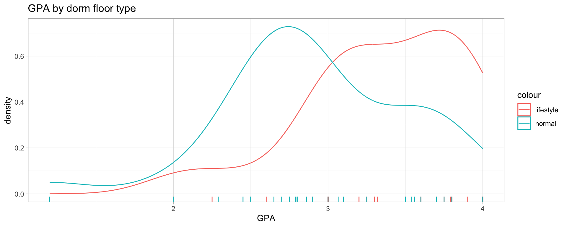
Recall the data on GPA by dorm floor from last lecture.

Code

dorm.gpa = tibble(
  lifestyle=c(2.00, 2.25, 2.60, 2.90, 3.00, 3.00, 3.00, 3.00, 3.00, 3.20, 
              3.20, 3.25, 3.30, 3.30, 3.32, 3.50, 3.50, 3.60, 3.60, 3.70, 
              3.75, 3.75, 3.79, 3.80, 3.80, 3.90, 4.00, 4.00, 4.00, 4.00),
  normal=c(1.20, 2.00, 2.29, 2.45, 2.50, 2.50, 2.50, 2.50, 2.65, 2.70, 
           2.75, 2.75, 2.79, 2.80, 2.80, 2.80, 2.86, 2.90, 3.00, 3.07, 
           3.10, 3.25, 3.50, 3.54, 3.56, 3.60, 3.70, 3.75, 3.80, 4.00)
)
ggplot(dorm.gpa) +
  geom_density(aes(x=lifestyle, color="lifestyle")) +
  geom_rug(aes(x=lifestyle, color="lifestyle")) +
  geom_density(aes(x=normal, color="normal")) +
  geom_rug(aes(x=normal, color="normal")) +
  labs(title="GPA by dorm floor type", x="GPA")

We can think of this data as a probabilistic model with predictor \(X=\{\text{lifestyle}, \text{normal}\}\) and response \(GPA\in[0,4]\).

Statistical Models

Our first step in analyzing this was with a two-sample T-test, an approach that assumes a normal error model, so that the complete model here would have been:

\[ GPA(X) = \begin{cases} \mu_{\text{lifestyle}} + \epsilon & \text{if }X = \text{lifestyle} \\ \mu_{\text{normal}} +\epsilon & \text{if }X = \text{normal} \end{cases} \qquad \epsilon\sim\mathcal{N}(0,\sigma^2) \]

An alternative way to write the same model could be:

\[ GPA(X) \sim \mathcal{N}(\mu(X), \sigma^2) \]

with the error terms taken as implicit.

The Simple Linear Regression Model

One step up in complexity from the functions of one or two distinct values we have seen previously would be a linear function¹: \(y = \beta_0+\beta_1x\).

We define:

Definition

The simple linear regression model is an additive model with one predictor and one response connected by a linear function and homoscedastic independent normal errors.

\[ Y = \beta_0 + \beta_1x + \epsilon \qquad \epsilon\sim\mathcal{N}(0,\sigma^2) \]

with deterministic predictor \(x\) without randomness or measurement error, and randomly varying \(Y\).

The population regression line is the line of expected values \(y = \beta_0+\beta_1x\).

1. The use of \(\beta_i\) for coefficients here is customary to statistical regression.

Exercise 12.9

Flow rate \(y\) (\(m^3/min\)) in a measurement device depends on the pressure drop \(x\) (inches of water) across the device’s filter.

For \(x\in[5,20]\), the variables follow a regression model with regression line \(y=-.12 + 0.095x\).

a. What is the expected change in flow rate associated with a 1-inch increase in pressure drop?

With a slope of \(0.095\), we expect for every \(1\) that is added to \(x\), we would add \(0.095\) to \(y\).

b. What change in flow rate can be expected when pressure drop decreases by 5 inches?

With a decrease of 5 inches, we would expect a change of \(\beta_1\cdot\Delta x=0.095\cdot(-5)=-.475\), so a decrease by \(.475\).

c. What is the expected flow rate for a pressure drop of 10 inches? A drop of 15 inches?

\(\EE[Y|x=10]= -.12+.095\cdot 10=0.830\) and \(\EE[Y|x=15]= -.12+.095\cdot 15=1.305\)

Exercise 12.9

d. Suppose \(\sigma=0.025\) and consider a pressure drop of 10 inches. Calculate \(\PP(Y>0.835)\) and \(\PP(Y>0.840)\).

Since for \(x=10\), we get the distribution \(Y\sim\mathcal{N}(0.830, 0.025^2)\), we may calculate \(\PP(Y>0.835) = 1-CDF_{\mathcal{N}(0.830,0.025^2)}(0.835) \approx 0.4207\) or 42.07%, and \(\PP(Y>0.840) = 1-CDF_{\mathcal{N}(0.830,0.025^2)}(0.840) \approx 0.3446\) or 34.46%.

e. Let \(Y_1\) be measured at \(x=10\) and \(Y_2\) at \(x=11\). Calculate \(\PP(Y_2 < Y_1)\).

We are sampling \(Y_1\sim\mathcal{N}(0.830, \sigma^2)\) and \(Y_2\sim\mathcal{N}(0.925, \sigma^2)\) independently, and need to compute the probability of \(Y_2<Y_1\).

\(Y_2 < Y_1\) precisely when \(0<Y_1-Y_2\), so we can consider the random variable \(Y_1-Y_2\sim\mathcal{N}(0.830-0.925, 2\sigma^2) = \mathcal{N}(-0.095, 2\cdot0.025^2)\) and look for the probability mass where this difference is \(>0\).

This leads us to compute the upper tail \(1-CDF_{\mathcal{N}(-0.095, 0.03535^2)}(0)\approx0.0036\) for a probability of \(0.36%\) for the lower observation exceeding the higher observation.

Estimating \(\beta_0\), \(\beta_1\), \(\sigma^2\)

Among all possible choices of straight line models that we could pick (\(\Omega = \underbrace{\RR}_{\beta_0} \times \underbrace{\RR}_{\beta_1} \times \underbrace{\RR_{\geq 0}}_{\sigma^2}\)), we need to find the best fit.

There are a number of ways to do this, but by far the most popular is the least squares method - partially because we then in most cases get a closed simple formula for the model parameters.

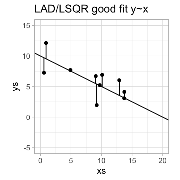
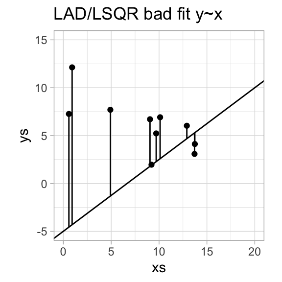
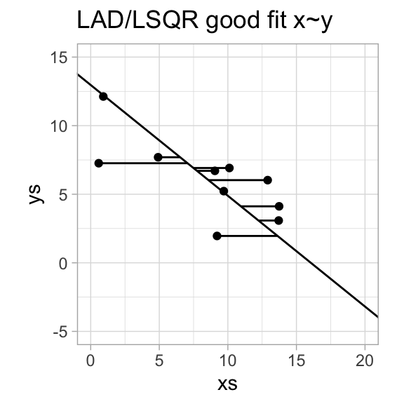
Measuring quality of fit

Least Absolute Deviations

Seek a regression function \(f\) that minimizes \(\sum_{i=1}^n|y_i-f(x_i)|\).

Iterative solutions with optimization methods.

Robust to outliers.

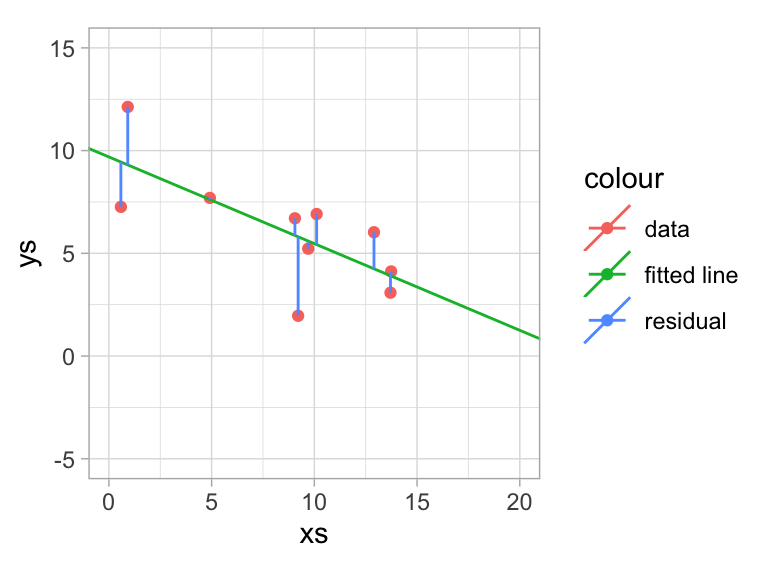
Least Squares

Seek a regression function \(f\) that minimizes \(\sum_{i=1}^n(y_i-f(x_i))^2\).

Unique (often) closed form solution.

Not robust.

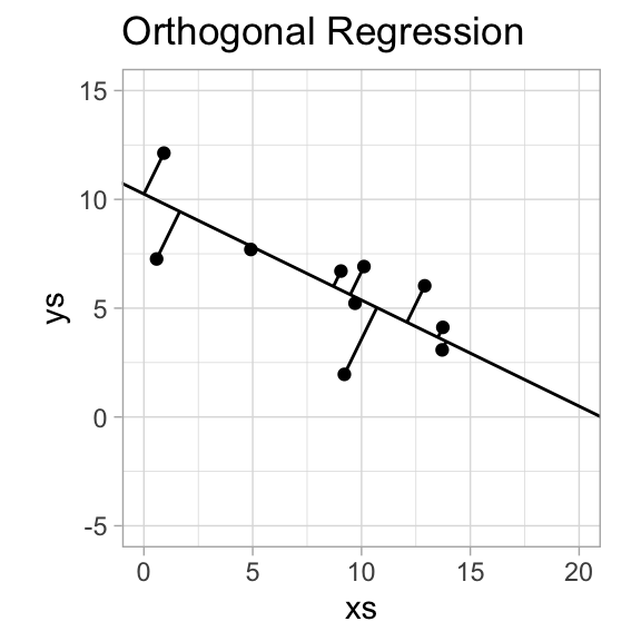
Orthogonal Regression

Seek a regression function \(f\) that minimizes shortest distance from data point to line.

Symmetric!

Measuring quality of fit

Code

b.0 = 10
b.1 = -.5
s = 2.5
a.0 = -5
a.1 = 0.75
df = tibble(xs = runif(10,0,20),
            ys = b.0 + b.1*xs + rnorm(10, sd=s),
            ypred = b.0 + b.1*xs,
            ybad = a.0 + a.1*xs)

pca = prcomp(~xs + ys, data=df, retx=T, center=T, scale=F)
orth = t(pca$x[,1] %*% t(pca$rotation[,1])) + pca$center
df$xorth = orth[1,]
df$yorth = orth[2,]
pca_b.1 = pca$rotation["ys","PC1"]/pca$rotation["xs","PC1"]
pca_b.0 = pca$center[2]-pca_b.1*pca$center[1]

xlm = lm(xs ~ ys, data=df)
df$xpred = predict(xlm, df)

ggplot(df) +
  geom_point(aes(x=xs, y=ys)) +
  geom_segment(aes(x=xs, xend=xs, y=ys, yend=ypred)) +
  geom_abline(aes(slope=b.1, intercept=b.0)) +
  coord_fixed(xlim=c(0,20), ylim=c(-5,15)) +
  labs(title="LAD/LSQR good fit y~x")
ggplot(df) +
  geom_point(aes(x=xs, y=ys)) +
  geom_segment(aes(x=xs, xend=xs, y=ys, yend=ybad)) +
  geom_abline(aes(slope=a.1, intercept=a.0)) +
  coord_fixed(xlim=c(0,20), ylim=c(-5,15)) +
  labs(title="LAD/LSQR bad fit y~x")
ggplot(df) +
  geom_point(aes(x=xs, y=ys)) +
  geom_segment(aes(x=xs, xend=xpred, y=ys, yend=ys)) +
  geom_abline(aes(slope=1/xlm$coefficients["ys"], intercept=-xlm$coefficients["(Intercept)"]/xlm$coefficients["ys"])) +
  coord_fixed(xlim=c(0,20), ylim=c(-5,15)) +
  labs(title="LAD/LSQR good fit x~y")
ggplot(df) +
  geom_point(aes(x=xs, y=ys)) +
  geom_segment(aes(x=xs, xend=xorth, y=ys, yend=yorth)) +
  geom_abline(aes(slope=pca_b.1, intercept=pca_b.0)) +
  coord_fixed(xlim=c(0,20), ylim=c(-5,15)) +
  labs(title="Orthogonal Regression")

Least Squares Estimation

We are trying to minimize the sum of squares of the residuals: \[ SSR = \sum(y_i - \hat y_i)^2 = \sum(y_i - f(x_i))^2 = \sum(y_i - (b_0 + b_1x_i))^2 \]

As usual, we compute partial derivatives with respect to the parameters \(b_0, b_1\) and seek critical values:

\[ \begin{align*} \frac{dSSR}{db_0} &= \sum 2(y_i-b_0-b_1x_i)\cdot(-1) & \frac{dSSR}{db_1} &= \sum 2(y_i-b_0-b_1x_i)\cdot(-x_i) \\ & \text{is zero when} && \text{is zero when} \\ \sum y_i &= n b_0 + b_1\sum x_i & \sum x_iy_i &= b_0 \sum x_i + b_1\sum x_i^2 \end{align*} \]

This is a system of linear equations in two unknowns (\(b_0, b_1\)), called the normal equations. As long as not all \(x_i\) are equal to each other, the system has a unique solution which provides the least squares estimate.

Least Squares Estimation

\[ \begin{align*} \sum y_i &= n b_0 + b_1\sum x_i & \sum x_iy_i &= b_0 \sum x_i + b_1\sum x_i^2 \\ b_0 &= \frac{\sum y_i}{n} - b_1\frac{\sum x_i}{n} = \overline{y}-b_1\overline{x} & \sum x_iy_i &= (\overline{y}-b_1\overline{x})\sum x_i + b_1\sum x_i^2 \\ && b_1 &= \frac{\sum x_iy_i - \overline{y}\sum x_i}{\sum x_i^2 - \overline{x}\sum x_i} \\ &&&= \frac{\sum x_iy_i - n\overline{x}\overline{y}}{\sum x_i^2-n\overline{x}^2} \\ &&&= \frac{\sum(x_i-\overline{x})(y_i-\overline{y})}{\sum(x_i-\overline{x})^2} \end{align*} \]

These estimates can be computed without actually computing each residual, by using: \[ S_{xy} = \sum x_iy_i-\frac{\left(\sum x_i\right)\left(\sum y_i\right)}{n} \quad S_{xx} = \sum x_i^2-\frac{\left(\sum x_i\right)^2}{n} \quad b_1=\hat\beta_1=\frac{S_{xy}}{S_{xx}} \]

Maximum Likelihood for Regression

(Exercise 12.23)

Find maximum likelihood estimates of \(\beta_0\) and \(\beta_1\) (and show that they are exactly what we derived).

Each \(Y_i\sim\mathcal{N}(\beta_0+\beta_1x_i, \sigma^2)\), so the joint likelihood is: \[ \begin{align*} \mathcal{L}(\beta_0,\beta_1,\sigma^2|y_1,\dots,y_n) &= \prod_i PDF_{\mathcal{N}(\beta_0+\beta_1x_i, \sigma^2)}(y_i) \\ &= \prod_i \frac{1}{\sqrt{2\pi\sigma^2}}\exp\left[-\frac{1}{2\sigma^2}(y_i-(\beta_0+\beta_1x_i))^2\right] \\ &\text{switching to log likelihood} \\ \ell(\beta_0,\beta_1,\sigma^2) &= \sum_i-\frac{1}{2}\left( \log(2\pi)+\log(\sigma^2)+\frac{1}{\sigma^2}(y_i-(\beta_0+\beta_1x_i))^2 \right) \\ &= -\frac{1}{2}\left( n\log(2\pi)+n\log(\sigma^2)+\frac{1}{\sigma^2}\sum(y_i-(\beta_0+\beta_1x_i))^2 \right) \end{align*} \]

Maximum Likelihood for Regression

(Exercise 12.23)

\[ \ell(\beta_0,\beta_1,\sigma^2) = -\frac{1}{2}\left( n\log(2\pi)+n\log(\sigma^2)+\frac{1}{\sigma^2}\sum(y_i-(\beta_0+\beta_1x_i))^2 \right) \\ \text{Take derivatives to find critical points} \\ \begin{align*} \frac{d\ell}{d\beta_0} &= -\frac{1}{2\sigma^2}\sum\left(2\cdot(y_i-(\beta_0+\beta_1x_i))\cdot(-1)\right) \\ \frac{d\ell}{d\beta_1} &= -\frac{1}{2\sigma^2}\sum\left(2\cdot(y_i-(\beta_0+\beta_1x_i))\cdot(-x_i)\right) \end{align*} \]

Extracting the factor \(-1/(2\sigma^2)\cdot 2\cdot (-1)\), we are left with the equations for critical points exactly matching the normal equations. So finding the MLEs proceeds identical to how we derived estimates from the normal equations before.

Estimating \(\sigma^2\)

Once we have estimated \(\hat\beta_0\) and \(\hat\beta_1\), we can compute fitted or predicted values \(\hat y_i = \hat\beta_0+\hat\beta_1x_i\). The residuals are the prediction errors \(e_i = y_i - \hat y_i\).

Key to estimating \(\sigma^2\) is a similar kind of separation of sources of variance as we saw in ANOVA.

The variance \(\VV[Y]\) comes in part from the slope of the line (spreading out the observations), and in part from the inherent variance \(\sigma^2\).

The residuals measure exactly the deviation that is not due to the slope of the regression line, so we may want to use the variance of the residuals to estimate \(\sigma^2\).

Estimating \(\sigma^2\)

Define \[ SSE = \sum e_i^2 = \sum(y_i-\hat y_i)^2 = \sum(y_i-(\hat\beta_0+\hat\beta_1x_i))^2 = \\ =\sum y_i^2 - \hat\beta_0\sum y_i - \hat\beta_1\sum x_iy_i \]

Since \(\overline e = 0\) (as we will prove in a little while), \(\frac{1}{n}\sum e_i^2\) is a (biased, consistent, MLE) estimator of \(\sigma^2\).

Because we have to estimate \(\hat\beta_0\) and \(\hat\beta_1\), the denominator needed for an unbiased variance estimate is \(n-2\):

\[ \hat\sigma^2 = s^2 = \frac{SSE}{n-2} \]

Coefficient of determination

Code

df1 = tibble(
  xs = seq(0,10,by=0.25),
  ys = 0.5*xs+2 + rnorm(length(xs), sd=0.05)
)
lm1 = lm(ys~xs, data=df1)
df1$ypred = predict(lm1, df1)

df2 = tibble(
  xs = seq(0,10,by=0.25),
  ys = 0.5*xs+2 + rnorm(length(xs), sd=0.5)
)
lm2 = lm(ys~xs, data=df2)
df2$ypred = predict(lm2, df2)

df3 = tibble(
  xs = seq(0,10,by=0.25),
  ys = 0.5*xs+2 + rnorm(length(xs), sd=2.5)
)
lm3 = lm(ys~xs, data=df3)
df3$ypred = predict(lm3, df3)



ggplot(df1, aes(xs,ys)) +
  geom_point() +
  geom_abline(slope=lm1$coefficients["xs"], intercept=lm1$coefficients["(Intercept)"]) +
  coord_fixed(ratio=0.5, xlim=c(0,10), ylim=c(-5,15)) + 
  labs(title=str_glue(
    "SST={round((nrow(df1)-1)*var(df1$ys),2)}, ",
    "SSE={round((nrow(df1)-1)*var(df1$ys-df1$ypred),4)}"
    ),
    subtitle=str_glue(
      "SSE/SST={round(100*var(df1$ys-df1$ypred)/var(df1$ys),2)}%"
    ))
ggplot(df2, aes(xs,ys)) +
  geom_point() +
  geom_abline(slope=lm2$coefficients["xs"], intercept=lm2$coefficients["(Intercept)"]) +
  coord_fixed(ratio=0.5, xlim=c(0,10), ylim=c(-5,15)) + 
  labs(title=str_glue(
    "SST={round((nrow(df2)-1)*var(df2$ys),2)}, ",
    "SSE={round((nrow(df2)-1)*var(df2$ys-df2$ypred),4)}"
    ),
    subtitle=str_glue(
      "SSE/SST={round(100*var(df2$ys-df2$ypred)/var(df2$ys),2)}%"
    ))
ggplot(df3, aes(xs,ys)) +
  geom_point() +
  geom_abline(slope=lm3$coefficients["xs"], intercept=lm3$coefficients["(Intercept)"]) +
  coord_fixed(ratio=0.5, xlim=c(0,10), ylim=c(-5,15)) + 
  labs(title=str_glue(
    "SST={round((nrow(df3)-1)*var(df3$ys),2)}, ",
    "SSE={round((nrow(df3)-1)*var(df3$ys-df3$ypred),4)}"
    ),
    subtitle=str_glue(
      "SSE/SST={round(100*var(df3$ys-df3$ypred)/var(df3$ys),2)}%"
    ))

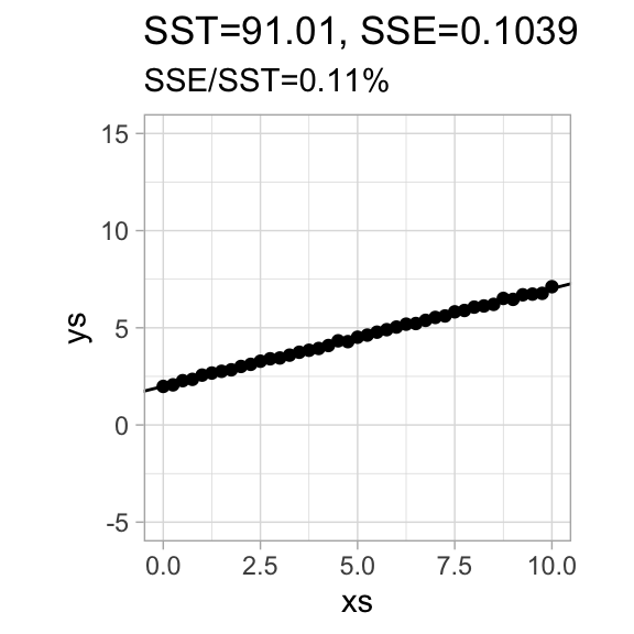
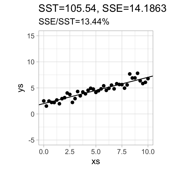
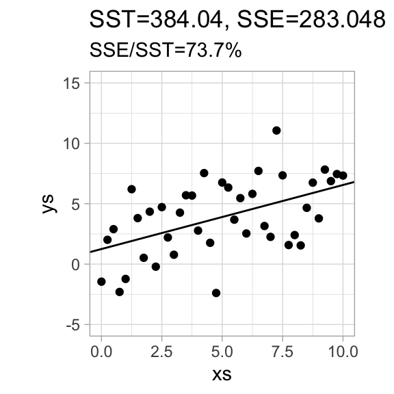
We define the coefficient of determination \(r^2 = 1 - \frac{SSE}{SST}\), the fraction of the total variance that is not explained by the variance of the residuals. The notation hints at a connection to correlations, which we will later see more about.

ANOVA Equation for Regression

(Exercise 12.24)

Write \(e_i=y_i-\hat y_i=y_i-(b_0+b_1x_i)\) for the residuals.

a.: Show \(\sum e_i=0\) and \(\sum e_ix_i=0\).

\[ \begin{align*} \sum e_i &= \sum (y_i-(b_0+b_1x_i)) & \sum x_ie_i &= \sum (y_i-(b_0+b_1x_i))x_i \\ &\propto \frac{dSSR}{db_0} = 0 & &\propto \frac{dSSR}{db_1} = 0 \end{align*} \]

b.: Show \(\hat y_i-\overline{y} = \hat\beta_1(x_i-\overline{x})\)

\[ \begin{align*} \hat y_i-\overline y &= \hat y_i - \frac{1}{n}\sum y_j = \hat y_i-\frac{1}{n}\sum (\hat y_j+e_j) \\ &= (\hat\beta_0 + \hat\beta_1x_i) - \frac{1}{n}\sum(\hat\beta_0+\hat\beta_1x_j)-\frac{1}{n}\sum e_j & \sum e_j &= 0 \quad\text{by the above} \\ &= \hat\beta_0 + \hat\beta_1x_i - \frac{1}{n} n\hat\beta_0 - \hat\beta_1\overline x = \hat\beta_1(x_i-\overline x) \end{align*} \]

ANOVA Equation for Regression

(Exercise 12.24)

c.: Derive \(SST = SSE + SSR\) for the linear model

We define the regression sum of squares \(SSR = \sum(\hat y_i-\overline y)^2\), and compute:

\[ \begin{align*} SST &= \sum(y_i - \overline y)^2 = \sum(\color{Teal}{(y_i-\hat y_i)} + \color{DarkMagenta}{(\hat y_i-\overline y)})^2 \\ &= \underbrace{\sum_i\color{Teal}{(y_i-\hat y_i)^2}}_{SSE} + 2\sum_i\color{Teal}{(y_i-\hat y_i)}\color{DarkMagenta}{(\hat y_i-\overline y)} + \underbrace{\sum_i\color{DarkMagenta}{(\hat y_i-\overline y)^2}}_{SSR} \end{align*} \]

Now note that \[ \begin{align*} \sum_i (y_i-\hat y_i)(\hat y_i-\overline y) &= \sum_i e_i\hat y_i - \overline y\sum_i e_i = \sum_i e_i(\hat\beta_0+\hat\beta_1x_i) - \overline y\cdot 0 \\ &= \hat\beta_0\sum_i e_i + \hat\beta_1\sum e_ix_i = \hat\beta_0\cdot0+\hat\beta_1\cdot 0 = 0 \end{align*} \]

ANOVA Equation for Regression

(Exercise 12.24)

d.: Verify \(SSE = \sum y_i^2 - \hat\beta_0\sum y_i - \hat\beta_1\sum x_iy_i\)

\[ \begin{align*} SSE &= \sum(y_i-\hat y_i)^2 \\ &= \sum\left((y_i-\overline y)-(\hat y_i-\overline y)\right)^2 \\ &= \sum((y_i-\overline y)-\hat\beta_1(x_i-\overline x))^2 \\ &= \sum\left((y_i-\overline y)^2 - 2\hat\beta_1(y_i-\overline y)(x_i-\overline x)+\hat\beta_1^2(x_i-\overline x)^2\right) \\ &= S_{yy} - 2\hat\beta_1S_{xy} + \hat\beta_1^2S_{xx} \qquad\text{recall:} \hat\beta_1=\frac{S_{xy}}{S_{xx}}\\ &= S_{yy}-2\hat\beta_1S_{xy}+\hat\beta_1S_{xy} = S_{yy}-\hat\beta_1S_{xy} \\ &= \sum y_i^2-2\overline y\underbrace{\sum y_i}_{=n\overline y} + n\overline y^2 - \hat\beta_1\sum x_iy_i +\hat\beta_1\overline y\underbrace{\sum x_i}_{=n\overline x} + \hat\beta_1\overline x\underbrace{\sum y_i}_{=n\overline y} - n\hat\beta_1\overline x\overline y \end{align*} \]

ANOVA Equation for Regression

(Exercise 12.24)

d.: Verify \(SSE = \sum y_i^2 - \hat\beta_0\sum y_i - \hat\beta_1\sum x_iy_i\)

\[ \begin{align*} SSE &= \sum y_i^2-2\overline y\underbrace{\sum y_i}_{=n\overline y} + n\overline y^2 - \hat\beta_1\sum x_iy_i +\hat\beta_1\overline y\underbrace{\sum x_i}_{=n\overline x} + \hat\beta_1\overline x\underbrace{\sum y_i}_{=n\overline y} - n\hat\beta_1\overline x\overline y \\ &= \sum y_i^2 - n\overline y^2 - \hat\beta_1\sum x_iy_i + n\hat\beta_1\overline x\overline y \\ &= \sum y_i^2 - \underbrace{n\overline y}_{=\sum y_i}\underbrace{(\overline y-\hat\beta_1\overline x)}_{=\hat\beta_0} - \hat\beta_1\sum x_iy_i \\ &= \sum y_i^2 - \hat\beta_0\sum y_i - \hat\beta_1\sum x_iy_i\qquad\text{QED} \end{align*} \]

Point of averages is on the regression line

Exercise 12.27

Often useful is the fact that \((\overline x, \overline y)\) is actually on the regression line directly, which we can see by computing:

\[ \hat\beta_0 + \hat\beta_1\overline x = \overline y - \hat\beta_1\overline x + \hat\beta_1\overline x = \overline y \]

Inferences about the slope

To build inferences (hypothesis tests and confidence intervals) about the slope \(\beta_1\) of a linear regression model, we will rephrase these results as claims about random variables.

We will not be working with random predictors here - the \(x_i\) are all deterministic, but instead of values \(y_i\) we will have random variables \(Y_i\) (and hence also \(\overline Y\) and \(S^2\)).

We note that \(S_{xY} = \sum(x_i-\overline x)(Y_i-\overline Y) = \sum Y_i(x_i-\overline x) - \overline Y\underbrace{\sum(x_i-\overline x)}_{=0}\).

It follows that \[ \hat\beta_1 = \sum\frac{(x_i-\overline x)}{S_{xx}}Y_i \qquad \hat\beta_0 = \frac{\sum Y_i - \hat\beta_1\sum x_i}{n} \qquad \hat\sigma^2 = \frac{\sum Y_i^2-\hat\beta_0\sum Y_i-\hat\beta_1\sum x_iY_i}{n-2} \]

Notice that this makes \(\hat\beta_1\) a sum of rescaled independent normal variables, so \(\hat\beta_1\) has a normal sampling distribution.

\(\hat\beta_1\) is unbiased

Exercise 12.40 a.

We check that:

\[ \begin{align*} \EE[\hat\beta_1] &= \EE\left[ \sum\frac{(x_i-\overline x)(Y_i-\overline Y)}{S_{xx}} \right] \\ &= \sum\frac{(x_i-\overline x)}{S_{xx}}(\EE[Y_i]-\EE[\overline Y]) \\ &= \sum\frac{(x_i-\overline x)}{S_{xx}}(\beta_0+\beta_1x_i-\beta_0-\beta_1\overline x) \\ &= \beta_1\sum\frac{(x_i-\overline x)}{S_{xx}}(x_i-\overline x) = \beta_1 \end{align*} \]

\(\hat\beta_0\) is unbiased

Exercise 12.39

We check that:

\[ \begin{align*} \EE[\hat\beta_0] &= \EE\left[\frac{\sum Y_i - \hat\beta_1\sum x_i}{n}\right] \\ &= \frac{\sum \EE[Y_i] - \EE[\hat\beta_1]\sum x_i}{n} \\ &= \frac{\sum(\beta_0+\beta_1x_i) - \beta_1\sum x_i}{n} \\ &= \frac{\sum\beta_0+\beta_1\sum x_i-\beta_1\sum x_i}{n} = \frac{n\beta_0}{n} = \beta_0 \end{align*} \]

Variance of \(\hat\beta_1\)

Exercise 12.40 b.

Here, it is easier to use the abbreviated formula for \(\hat\beta_1\). We check:

\[ \begin{align*} \VV[\hat\beta_1] &= \VV\left[ \sum\frac{(x_i-\overline x)}{S_{xx}}Y_i \right] \\ &= \sum\frac{(x_i-\overline x)^2}{S_{xx}^2}\VV[Y_i] \\ &= \frac{S_{xx}}{S_{xx}^2}\sigma^2 = \frac{\sigma^2}{S_{xx}} \end{align*} \]

A T-distribution for \(\hat\beta_1\)

Since the standard error for the estimator \(\hat\beta_1\) is \(\sigma/\sqrt{S_{xx}}\), and since the \(S^2=SSE/(n-2)\) estimator has \(n-2\) degrees of freedom, we get that:

\[ \frac{\hat\beta_1-\beta_1}{\sigma/\sqrt{S_{xx}}}\sim\mathcal{N}(0,1) \qquad \frac{(n-2)S^2}{\sigma^2}\sim\chi^2(n-2) \qquad \frac {\frac{\hat\beta_1-\beta_1}{\sigma/\sqrt{S_{xx}}}} {\sqrt{\frac{(n-2)S^2}{\sigma^2}/(n-2)}}\sim T(n-2) \]

We can simplify:

\[ \frac {\frac{\hat\beta_1-\beta_1}{\sigma/\sqrt{S_{xx}}}} {\sqrt{\frac{\color{DarkMagenta}{(n-2)}S^2}{\sigma^2}/\color{DarkMagenta}{(n-2)}}} = \frac{\hat\beta_1-\beta_1}{\color{DarkMagenta}{\sigma}/\sqrt{S_{xx}}}\cdot\frac{\color{DarkMagenta}{\sigma}}{S} = \frac{\hat\beta_1-\beta_1}{S/\sqrt{S_{xx}}} \]

T-Test and Confidence Interval for \(\hat\beta_1\)

T-Test for linear regression

Null Hypothesis

\(\beta_1=\beta_{10}\), often taken as \(0\) (for the model utility test - checking whether the model does anything useful at all)

Test Statistic

\(t=\frac{\hat\beta_1-\beta_{10}}{s/\sqrt{s_{xx}}}\)

Alternative Hypothesis	Rejection Region for Level \(\alpha\)	p-value
Upper Tail	\(t\geq t_{\alpha,n-2}\)	\(1-CDF_{T(n-2)}(t)\)
Two-tailed	\(|t|\geq t_{\alpha/2,n-2}\)	\(\min\{CDF_{T(n-2)}(t), 1-CDF_{T(n-2)}(t)\}\)
Lower Tail	\(t\leq -t_{\alpha,n-2}\)	\(CDF_{T(n-2)}(t)\)

\(1-\alpha\) Confidence Interval

\(\beta_1\in\hat\beta_\pm t_{\alpha/2,n-2}s/\sqrt{s_{xx}}\)

ANOVA F-Test for Linear Regression

The model utility test can equivalently be tested with an ANOVA approach - and doing this sets the stage for easier generalization to multilinear regression (not in scope for this course):

ANOVA table for simple linear regression

Source	Sum of Squares	DoF	Mean Square	F	p
Regression	SSR	1	SSR	\(\frac{SSR}{SSE/(n-2)}\)	\(1-CDF_{F(1,n-2)}(F)\)
Error	SSE	\(n-2\)	\(s^2=\frac{SSE}{n-2}\)
Total	SST	\(n-1\)