ANOVA
\[ \def\RR{{\mathbb{R}}} \def\PP{{\mathbb{P}}} \def\EE{{\mathbb{E}}} \def\VV{{\mathbb{V}}} \]
ANOVA with 2 Factor Levels
When we are testing exactly 2 groups, with \(I=2\), the ANOVA F-test hypotheses reduce to: \[ H_0:\mu_1=\mu_2 \qquad H_a:\mu_1\neq\mu_2 \]
The test statistic for the T-test is: \[ T = \frac{Z}{\sqrt{X/\nu}} \qquad Z\sim\mathcal{N}(0,1) \qquad X\sim\chi^2(\nu) \]
Consider \(T^2\):
- Numerator
- Standard normal variable, squared. This has distribution \(\chi^2(1)\).
- Denominator
- Chi-squared variable divided by its degrees of freedom.
So \(T^2\sim F(1,\nu)\).
ANOVA with 2 Factor Levels
As long as we are testing two-tailed T-tests, the ANOVA F and the Student’s T are equivalent. However:
| Student’s T | ANOVA F | |
|---|---|---|
| One-sided test? | ||
| Requires normality | Robust | Sensitive |
| Requires equal variances |
ANOVA with unequal sample sizes
Suppose groups have sizes \(J_1,\dots,J_I\). Write \(n=\sum J_i\). We write \(\overline{X}_{i,*}\), \(\overline{X}_{*,j}\) and \(\overline{X}_{*,*}\) for groupwise or overall means and \(X_{i,*}\), \(X_{*,i}\) and \(X_{*,*}\) for corresponding sums
| Source | SS* | Easy computation | DoF |
|---|---|---|---|
| Total | \(\sum_{i=1}^I\sum_{j=1}^{J_i}(X_{i,j}-\overline{X}_{*,*})^2\) | \(\sum_{i=1}^I\sum_{j=1}^{J_i}X_{i,j}^2 - \frac{1}{n}X_{*,*}^2\) | \(n-1\) |
| Treatment | \(\sum_{i=1}^I\sum_{j=1}^{J_i}(\overline{X}_{i,*}-\overline{X}_{*,*})^2\) | \(\sum_{i=1}^I \frac{1}{J_i}X_{i,*}^2 - \frac{1}{n}X_{*,*}^2\) | \(I-1\) |
| Error | \(\sum_{i=1}^I\sum_{j=1}^{J_i}(X_{i,j}-\overline{X}_{i,*})^2\) | \(SST-SSTr\) | \(\sum(J_i-1) = n-I\) |
Post-hoc Testing and Multiple Hypotheses
Recall that the one-way ANOVA null hypothesis is \(H_0:\mu_1=\dots=\mu_I\), for \(I\) distinct groups. Importantly, the ANOVA test does not itself tell us anything about which groups are different from other groups.
To uncover concrete differences, we would have to revert to pair-wise testing with two-sample T-tests. Doing so exposes us to the Multiple Hypothesis problem.
At the core of the problem is that if each individual test produces a false discovery with probability \(\alpha\), then performing several of them will raise the probability of false discovery.
Post-hoc Testing and Multiple Hypotheses

Tukey’s Method
Our book, in Chapter 11.2, describes Tukey’s procedure (aka Tukey’s Test, Tukey’s honest significance test, Tukey’s honest significant difference test). The test is rooted in deriving the studentized range distribution to describe the range of the means that occur:
Theorem
Let \(Z_1,\dots,Z_m\sim\mathcal{N}(0,1)\) iid, and \(W\sim\chi^2(\nu)\) independent from all these. Then the distribution of \[ Q = \frac{\max_i\{Z_i\}-\min_i\{Z_i\}}{\sqrt{W/\nu}} \sim Q(m, \nu) \]
This distribution is called the studentized range distribution or Tukey’s Q
This distribution is covered by the ptukey and qtukey functions in R, and by scipy.stats.studentized_range in Python.
Tukey’s Method
In an ANOVA context, we would choose: \[ Z_i = \frac{\overline{X}_{i,*}-\mu}{\sigma/\sqrt{J}} \qquad m=I \qquad W=\frac{SSE}{\sigma^2} = \frac{I(J-1)MSE}{\sigma^2} \qquad \nu=I(J-1) \\ Q = \frac{\overline{X}_\max-\overline{X}_\min}{\sqrt{MSE/J}} \]
Tukey’s Method
Picking \(q_{\alpha, I, I(J-1)} = CDF_{Q(I, I(J-1))}^{-1}(1-\alpha)\), each pairwise comparison of means has a confidence interval:
\[ \begin{align*} \overline{x}_{i,*}-\overline{x}_{j,*} \pm \frac{q_{\alpha, I, I(J-1)}}{\sqrt{MSE/J}} \end{align*} \]
The simultaneous confidence level for all these confidence intervals is \(1-\alpha\). Each interval that does not include 0 yields a conclusion of significant difference for that pair.
Equal Sized Groups
Most uses of Tukey’s method assume equal size groups in the data. If the sizes differ, you will need the Tukey-Kramer method instead.
Tukey’s Method
On the story chains data
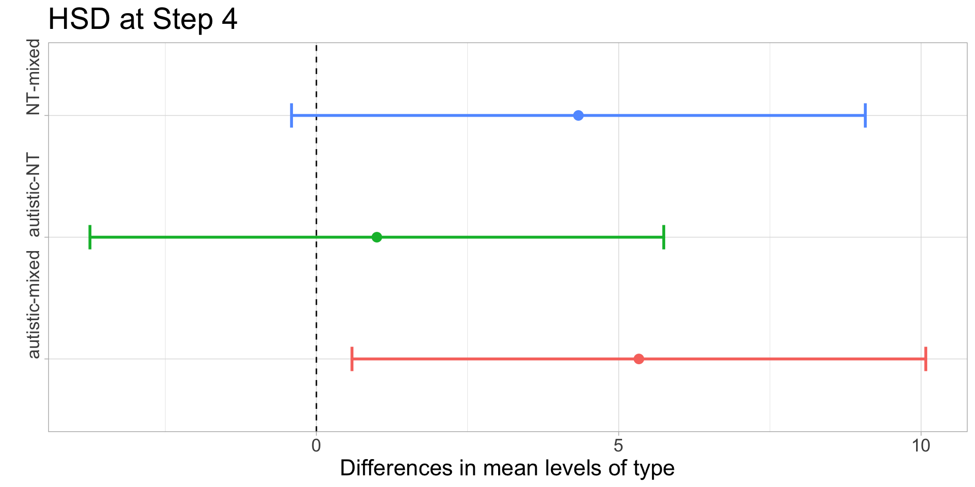
In order to illustrate what a significant result looks like, I have chosen \(\alpha=0.10\) for this example. With \(I=3\) and \(J=3\) we get \(\nu=6\) and \(q_{0.10,3,6}\approx 3.56\). Recall that the group means were:
| Step | \(\overline{X}_{NT}\) | \(\overline{X}_{mixed}\) | \(\overline{X}_{autistic}\) | MSE |
|---|---|---|---|---|
| 4 | 12.67 | 8.33 | 13.67 | 5.33 |
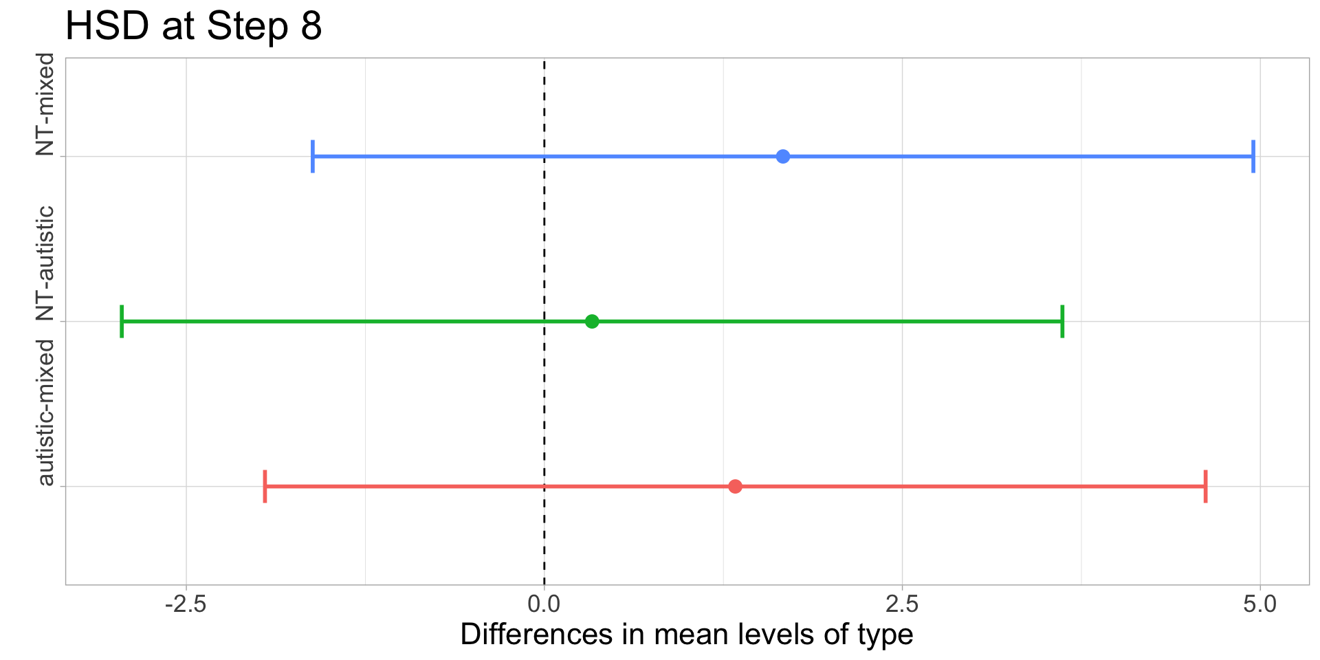
| 8 | 6 | 4.33 | 5.67 | 2.56 |
Compute the honestly significantly difference \(q_{0.10,3,6}\cdot\sqrt{MSE/J}\) - for step 4, \(\approx 3.56\cdot\sqrt{5.33/3}\approx 4.74\) and for step 8, \(\approx 3.56\cdot\sqrt{2.56/3}\approx 3.29\).
At Step 8, all three groups are not significantly different (since 6-4.33=1.67<3.29), but at Step 4, the difference between autistic and mixed is significant (5.34>4.74), and the difference between NT and mixed just barely misses the significance threshold (4.34<4.74).
Tukey’s Method
On the story chains data
Code
| step | NT | autistic | mixed | hsd |
|---|---|---|---|---|
| 4 | 12.67 | 13.67 | 8.33 | 4.74 |
| 8 | 6.00 | 5.67 | 4.33 | 3.28 |
CIs from pairwise differences of means and Tukey’s margin of error:
Code
inner_join(group.means, hsd) %>%
  mutate(`NT-autistic`=NT-autistic,
         `NT-mixed`=NT-mixed,
         `autistic-mixed`=autistic-mixed) %>%
  select(step,`NT-autistic`,`NT-mixed`,`autistic-mixed`,hsd) %>%
  pivot_longer(contains("-"), names_to="comparison", values_to="mean.diff") %>%
  transmute(step, comparison, lo=mean.diff-hsd, hi=mean.diff+hsd) %>%
  pivot_wider(names_from="step", values_from=c("lo","hi")) %>%
  select(comparison,
         `step 4: CI low`=lo_4, `step 4: CI high`=hi_4,
         `step 8: CI low`=lo_8, `step 8: CI high`=hi_8) %>%
kable()| comparison | step 4: CI low | step 4: CI high | step 8: CI low | step 8: CI high |
|---|---|---|---|---|
| NT-autistic | -5.7444955 | 3.744496 | -2.950895 | 3.617562 |
| NT-mixed | -0.4111621 | 9.077829 | -1.617562 | 4.950895 |
| autistic-mixed | 0.5888379 | 10.077829 | -1.950895 | 4.617562 |
Tukey’s Method
In R
First perform the ANOVA with aov.
Code
story.last = story.chains[c(4,8),] %>%
  pivot_longer(starts_with("chain"), names_to="chain", values_to="retained") %>%
  inner_join(chain.type, by="chain")
model.4 = aov(retained ~ type, story.last %>% filter(step==4))
model.8 = aov(retained ~ type, story.last %>% filter(step==8))
TukeyHSD(model.4, ordered=TRUE, conf.level=0.90)
TukeyHSD(model.8, ordered=TRUE, conf.level=0.90)
Tukey multiple comparisons of means
90% family-wise confidence level
factor levels have been ordered
Fit: aov(formula = retained ~ type, data = story.last %>% filter(step == 4))
$type
diff lwr upr p adj
NT-mixed 4.333333 -0.4111621 9.077829 0.1320774
autistic-mixed 5.333333 0.5888379 10.077829 0.0673680
autistic-NT 1.000000 -3.7444955 5.744495 0.8597820 Tukey multiple comparisons of means
90% family-wise confidence level
factor levels have been ordered
Fit: aov(formula = retained ~ type, data = story.last %>% filter(step == 8))
$type
diff lwr upr p adj
autistic-mixed 1.3333333 -1.950895 4.617562 0.5914726
NT-mixed 1.6666667 -1.617562 4.950895 0.4566371
NT-autistic 0.3333333 -2.950895 3.617562 0.9648950Tukey’s Method
In R
Tukey’s Method
In Python
In scipy.stats there is a function tukey_hsd that computes the honestly significant differences for us. Like the f_oneway function, it takes
Code
Tukey's HSD Pairwise Group Comparisons (95.0% Confidence Interval)
Comparison  Statistic  p-value  Lower CI  Upper CI
 (0 - 1)      4.333     0.132    -1.452    10.119
 (0 - 2)     -1.000     0.860    -6.786     4.786
 (1 - 0)     -4.333     0.132   -10.119     1.452
 (1 - 2)     -5.333     0.067   -11.119     0.452
 (2 - 0)      1.000     0.860    -4.786     6.786
(2 - 1) 5.333 0.067 -0.452 11.119ConfidenceInterval(low=array([[ -4.74449546, -0.41116213, -5.74449546],
[ -9.07782879, -4.74449546, -10.07782879],
[ -3.74449546, 0.58883787, -4.74449546]]), high=array([[ 4.74449546, 9.07782879, 3.74449546],
[ 0.41116213, 4.74449546, -0.58883787],
[ 5.74449546, 10.07782879, 4.74449546]]))p-values for pairwise comparisons
The upcoming methods all deal with modifying p-values or p-value comparison targets. For our running example, we will therefore here compute the pair-wise 2-sample p-values to keep using it as a running example:
Code
NT_autistic = scipy.stats.ttest_ind(NT, autistic, equal_var=False)
NT_mixed = scipy.stats.ttest_ind(NT, mixed, equal_var=False)
autistic_mixed = scipy.stats.ttest_ind(autistic, mixed, equal_var=False)

print(f"""
Comparison | p
-|-
NT vs autistic | {NT_autistic.pvalue:.4f}
NT vs mixed | {NT_mixed.pvalue:.4f}
autistic vs mixed | {autistic_mixed.pvalue:.4f}
""")| Comparison | p |
|---|---|
| NT vs autistic | 0.6984 |
| NT vs mixed | 0.0107 |
| autistic vs mixed | 0.1318 |
Bonferroni’s Method
Bonferroni’s method is based on the observation that the probability of rejecting any one null hypothesis in error, if each hypothesis test is run at a level of \(\alpha_c\), would be \[ \PP(p_1\leq\alpha_c \text{ or }\dots\text{ or }p_m\leq\alpha_c) \leq \sum_i\PP(p_i\leq\alpha_c) \leq m\alpha_c \]
The Bonferroni correction achieves an overall test level \(\alpha\) for \(m\) simultaneous hypotheses by picking a level for each test of \(\alpha/m\).
Dunn extended the procedure to confidence intervals by suggesting that each confidence interval be computed at a confidence level \(1-\alpha/m\) to achieve an overall confidence level of \(1-\alpha\).
Bonferroni’s Method
Warning
Even though Bonferroni’s method is very simple, and therefore widely spread, it is known to be conservative: the inequalities used to derive the bound hold for disjoint events, and it is unlikely that this assumption would hold.
So using \(\alpha/m\) instead of \(\alpha\) is likely to make you work harder (do more experiments) than you might have needed to.
Running Example
At an overall \(\alpha=0.10\), we would here choose to reject whenever p-values are less than \(\alpha/m=0.10/3\approx0.033\).
Code
| Comparison | p | Reject? |
|---|---|---|
| NT vs autistic | 0.6984 | False |
| NT vs mixed | 0.0107 | True |
| autistic vs mixed | 0.1318 | False |
Holm’s Method
Given \(m\) simultaneous hypotheses that you test separately producing p-values \(p_i\). We will be working with the sorted p-values \(p_{(1)}\leq p_{(2)}\leq\dots\leq p_{(m)}\).
With Holm’s method you go through the p-values in ascending order, and at each step compare:
As there are \(m+1-k\) p-values left to compare at step \(k\) (including the current one), compare \(p_{(k)} < \frac{\alpha}{m+1-k}\).
Repeat this step until the first time you are unable to reject the null hypothesis, and fail to reject all the later occurring null hypotheses.
Holm’s Method
Running Example
| Comparison | p | Compare against | Reject? |
|---|---|---|---|
| NT vs mixed | 0.0107 | 0.0333 | True |
| autistic vs mixed | 0.1318 | 0.0500 | False |
| NT vs autistic | 0.6984 | 0.1000 | False |
Since the first non-rejection happens at step 2, we reject only step 1, and fail to reject steps 2 and 3.
Hochberg’s Method
(aka Benjamini-Hochberg’s Method)
For a target level \(\alpha\), and sorted p-values \(p_{(1)}\leq\dots\leq p_{(m)}\), find the largest \(k\) such that \(p_{(k)}\leq\frac{k}{m}\alpha\).
Reject hypotheses corresponding to \(p_{(1)},\dots,p_{(k)}\).
Hochberg’s method can be done graphically by plotting the sorted p-values against their indices \(1,\dots,m\) as well as a line through the origin with slope \(\alpha/m\). Rejection happens for all points that are to the left of the last point below the line.
Hochberg’s Method
Code
library(ggeasy)

story.last.4 = story.last %>% filter(step==4) %>%
  pivot_wider(values_from=retained, names_from=type)
NT.aut = t.test(story.last.4$NT, story.last.4$autistic)
NT.mix = t.test(story.last.4$NT, story.last.4$mixed)
aut.mix = t.test(story.last.4$autistic, story.last.4$mixed)
p.vals = c(NT.aut$p.value, NT.mix$p.value, aut.mix$p.value)

p.df = tibble(
  comparison=c("NT vs autistic", "NT vs mixed", "autistic vs mixed"),
  p.vals = p.vals
) %>% arrange(p.vals) %>% mutate(k=row_number())

ggplot(p.df) +
  geom_point(aes(x=k,y=p.vals)) +
  geom_abline(slope=0.10/nrow(p.df)) +
  ylim(0,1) +
  scale_x_continuous(breaks=p.df$k, labels=p.df$comparison, limits=c(0,4)) +
  easy_rotate_x_labels(angle=30, side="right")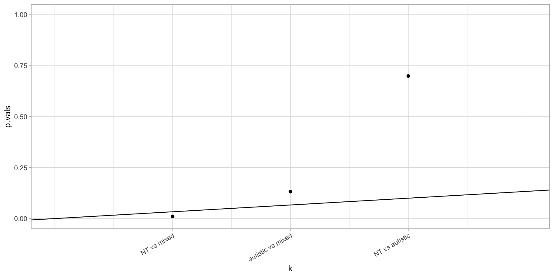
Storey-Tibshirani’s Method
Shifting focus from false positive rate to false discovery rate, John D Storey introduced the q-value in 2002 to control FDR for large sets of simultaneous tests.
False Discovery Rate is the ratio \(\frac{\#\text{false positives}}{\#\text{positives}}\). We write \(F\) for the number of false positives and \(S\) for the number of significant outcomes (ie positives). We want to pick a threshold \(t\) so that \[ FDR(t) = \EE\left[ \frac{F(t)}{S(t)} \right] \approx \frac{\EE[F(t)]}{\EE[S(t)]} \leq \alpha \]
Suppose we are performing \(m\) different hypothesis tests, with p-values \(p_1,\dots,p_m\). Depending on the threshold \(t\) that we pick we reject the null hypothesis for some number of these p-values. We can estimate \(\hat{S}(t)=\#\{p_i\leq t\}\).
Storey-Tibshirani’s Method
To estimate the expected number of false positives for some threshold \(t\), we can use the fact that under the null hypothesis, we expect p-values to distribute uniformly on \([0,1]\). We might expect \(m_0\cdot t\) of the outcomes to be false positives, where \(m_0\) is the total number of truly null features.
But \(m_0\) as well as the proportion \(\pi_0=m_0/m\) of features that are truly null, are both difficult to estimate. So instead, we may estimate the overall proportion of null p-values by \[ \hat\pi(\lambda) = \frac{\#\{p_i>\lambda\}}{m(1-\lambda)} \] with a tuning parameter \(\lambda\) that marks where we expect p-values to be primarily noise-driven.
Storey-Tibshirani’s Method
We can then estimate \(FDR\) by \[ \widehat{FDR}(t) = \frac{\hat\pi_0 m t}{\hat S(t)} = \frac{\hat\pi_0 m t}{\#\{p_i\leq t\}} \]
The \(q\)-value is then defined and estimated by: \[ q(p_i) = \min_{t\geq p_i}FDR(t) \qquad \hat{q}(p_i) = \min_{t\geq p_i}\widehat{FDR}(t) \]
Storey-Tibshirani’s Method
How to use it
- Python
- There is a package on GitHub that computes them: https://github.com/nfusi/qvalue
- R
-
The package
qvaluecomputes q-values from lists of p-values.
If you choose to reject every null hypothesis that has a q-value of no more than \(\alpha\), you should expect \(\alpha\) of the rejected null hypotheses to be rejected in error.
Software implementations
The library statsmodels has implementations of most p-value-based multiple hypothesis correction methods in statsmodels.stats.multitest.multipletests:
multipletests(p_vals.p_val, method="bonferroni", alpha=0.10)
multipletests(p_vals.p_val, method="holm", alpha=0.10)
multipletests(p_vals.p_val, method="simes-hochberg", alpha=0.10)- Bonferroni
- NT vs autistic: Fails to reject
- NT vs mixed: Rejects
- autistic vs mixed: Fails to reject
- Holm
- NT vs autistic: Fails to reject
- NT vs mixed: Rejects
- autistic vs mixed: Fails to reject
- Simes-Hochberg
- NT vs autistic: Fails to reject
- NT vs mixed: Rejects
- autistic vs mixed: Fails to reject
The function p.adjust produces adjusted p-values that can be compared to your required baseline level to decide on rejection or non-rejection.
Code
| comparisons | raw | bonferroni | holm | hochberg |
|---|---|---|---|---|
| NT vs. autistic | 0.6984 | 1.0000 | 0.6984 | 0.6984 |
| NT vs. mixed | 0.0107 | 0.0321 | 0.0321 | 0.0321 |
| Autistic vs. mixed | 0.1318 | 0.3953 | 0.2635 | 0.2635 |
Your Homework
10:48 - Nicholas Basile
\[ H_0: p_1-p_2 = 0 \qquad H_a:p_1-p_2 < 0 \qquad \alpha=.01 \\ z = {\hat p_1-\hat p_2 \over \sqrt{\hat p\hat q\left(\frac{1}{m}+\frac{1}{n}\right)}} = {\frac{x}{m}-\frac{\color{DarkMagenta}{y}}{n} \over \sqrt{\left(x+y\over m+n\right)\left(1-{x+y\over m+n}\right)\left(\frac{1}{m}+\frac{1}{n}\right)} } = \\ = {\frac{30}{200}-\frac{180}{600} \over \sqrt{\left(30+180\over 200+600\right)\left(1-{30+180\over 200+600}\right)\left(\frac{1}{200}+\frac{1}{600}\right)} } \approx -4.1753 \\ -z_{.01} \approx -2.32635 \geq z \Rightarrow \text{reject }H_0 \]
10:50 - MVJ
3 submissions. 3 different values for \(z\). I’m taking this one.
\[ H_0: p_p-p_s = 0 \qquad H_a: p_p - p_s < 0 \qquad \alpha=0.10 \\ \hat p_p = {104\over 207} \approx 0.5024 \qquad \hat p_s = {109\over 213} \approx 0.5117 \qquad \hat p = {104+109 \over 207+213} = {213\over 420} \approx 0.5071 \\ z = {\hat p_p - \hat p_s \over \sqrt{\hat p\hat q\left(\frac{1}{n_p}+\frac{1}{n_s}\right)}} = {\frac{104}{207} - \frac{109}{213} \over \sqrt{{213\over 420}\cdot{207\over 420}\cdot\left(\frac{1}{207}+\frac{1}{213}\right)}} \approx -.191036 \\ p = \Phi(z) \approx .424285 \]
Since the p-value exceeds \(\alpha\), we fail to reject the null hypothesis.
As a result we do not have data that supports claiming that return rates are lower for plain covers.
(if you came out with \(z\approx -.184\) or \(z\approx -.2049\) you have rounding errors from premature rounding that propagate through the computation)
10:62 - Victoria Paukova
From Exercise 27, \(m=10\), \(s_1=2.7508\), \(n=5\), \(s_2=4.4385\). We use \(\alpha=.1\).
\[ H_0: \sigma_1^2=\sigma_2^2 \qquad H_a: \sigma_1^2\neq \sigma_2^2 \\ f = {s_1^2\over s_2^2}\approx .3841 \]
We reject if \(f\geq F_{\alpha/2,m-1,n-1}\), \(f\leq F_{1-\alpha/2,m-1,n-1}\).
\[ F_{.05,9,4} \approx 5.9988 \qquad F_{.95,9,4} = {1\over F_{.05,4,9}} \approx {1\over 3.6331} \approx .275 \]
Since our f-value of \(.3841\) is not greater than \(5.9988\) nor less than \(.275\), we do not reject the null hypothesis, and conclude that there is not a difference between the standard deviations.
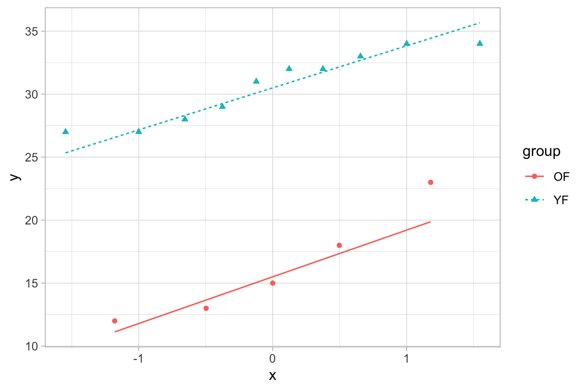
MVJ: For the F-test, we require that both samples are approximately normal. So the requisite normal probability plots would be a separate one for each sample. See Example 10.14 in the book for another example of this.
Here, we would get:
10:68 - Victoria Paukova
A 90% CI means we get to reuse the same values from above (\(\alpha=.1\))
\[ \left( {s_1\over s_2}{1\over\sqrt{F_{\alpha/2,m-1,n-1}}}, {s_1\over s_2}{1\over\sqrt{F_{1-\alpha/2,m-1,n-1}}} \right) \\ \left( {2.7508\over 4.4385}{1\over\sqrt{5.9988}}, {2.7508\over 4.4385}\sqrt{3.6331} \right) \approx (.253, 1.181) \]
This interval includes 1, which means we’re 90% confident that the ratio between the s values is 1 (no difference between them).
MVJ: Well, not quite. We are 90% confident that the ratio of standard deviations falls within a range that includes 1. This means that we do not have significant support for claiming that the ratio could not be 1.
10:78 - MVJ
Code
scores = pd.DataFrame({
  "score": [34,27,26,33,23,37,24,34,22,23,32, 5,
            30,35,28,25,37,28,26,29,22,33,31,23,
            37,29, 0,30,34,26,28,27,32,29,31,33,
            28,21,34,29,33, 6, 8,29,36, 7,21,30,
            28,34,28,35,30,34, 9,38, 9,27,25,33,
            9 ,23,32,25,37,28,23,26,34,32,34, 0,
            24,30,36,28,38,35,16,37,25,34,38,34,31, # end of E
            37,22,29,29,33,22,32,36,29, 6, 4,37,
            0 ,36, 0,32,27, 7,19,35,26,22,28,28,
            32,35,28,33,35,24,21, 0,32,28,27, 8,
            30,37, 9,33,30,36,28, 3, 8,31,29, 9,
            0 , 0,35,25,29, 3,33,33,28,32,39,20,
            32,22,24,20,32, 7, 8,33,29, 9, 0,30,
            26,25,32,38,22,29,29],
  "group": ["E"]*85 + ["C"]*79
})
a.: Determine a 95% CI for the difference of population means using the \(z\) method in Section 10.1.
We need to compute:
Code
sem2_E = scores.query("group=='E'").score.sem()**2
sem2_C = scores.query("group=='C'").score.sem()**2
margin = scipy.stats.norm.isf(.025)*np.sqrt(sem2_E+sem2_C)
ci_lo = scores.query("group=='E'").score.mean() - scores.query("group=='C'").score.mean() - margin
ci_hi = scores.query("group=='E'").score.mean() - scores.query("group=='C'").score.mean() + margin

print(f"""
$\\overline{{e}}$ | $\\overline{{c}}$ | $s_e^2$ | $s_c^2$ | $z_{{\\alpha/2}}$ | Margin | CI low | CI high
-|-|-|-|-|-|-|-|-|-
{scores.query("group=='E'").score.mean():.2f} | {scores.query("group=='C'").score.mean():.2f} | {scores.query("group=='E'").score.var():.2f} | {scores.query("group=='C'").score.var():.2f} | {scipy.stats.norm.isf(.025):.2f} | {margin:.2f} | {ci_lo:.2f} | {ci_hi:.2f}
""")| \(\overline{e}\) | \(\overline{c}\) | \(s_e^2\) | \(s_c^2\) | \(z_{\alpha/2}\) | Margin | CI low | CI high | ||
|---|---|---|---|---|---|---|---|---|---|
| 27.34 | 23.87 | 78.28 | 134.50 | 1.96 | 3.17 | 0.29 | 6.64 |
10:78 - MVJ
b.: Obtain a bootstrap sample of 999 differences of means. Check the bootstrap distribution for normality using a normal probability plot.
Code
import probscale # probability plots in matplotlib

bs_samples = [
  scores.query("group == 'E'").sample(frac=1.0, replace=True).score.mean() -
  scores.query("group == 'C'").sample(frac=1.0, replace=True).score.mean()
  for _ in range(999)]

probscale.probplot(bs_samples, plottype="prob", problabel="Standard Normal Probabilities")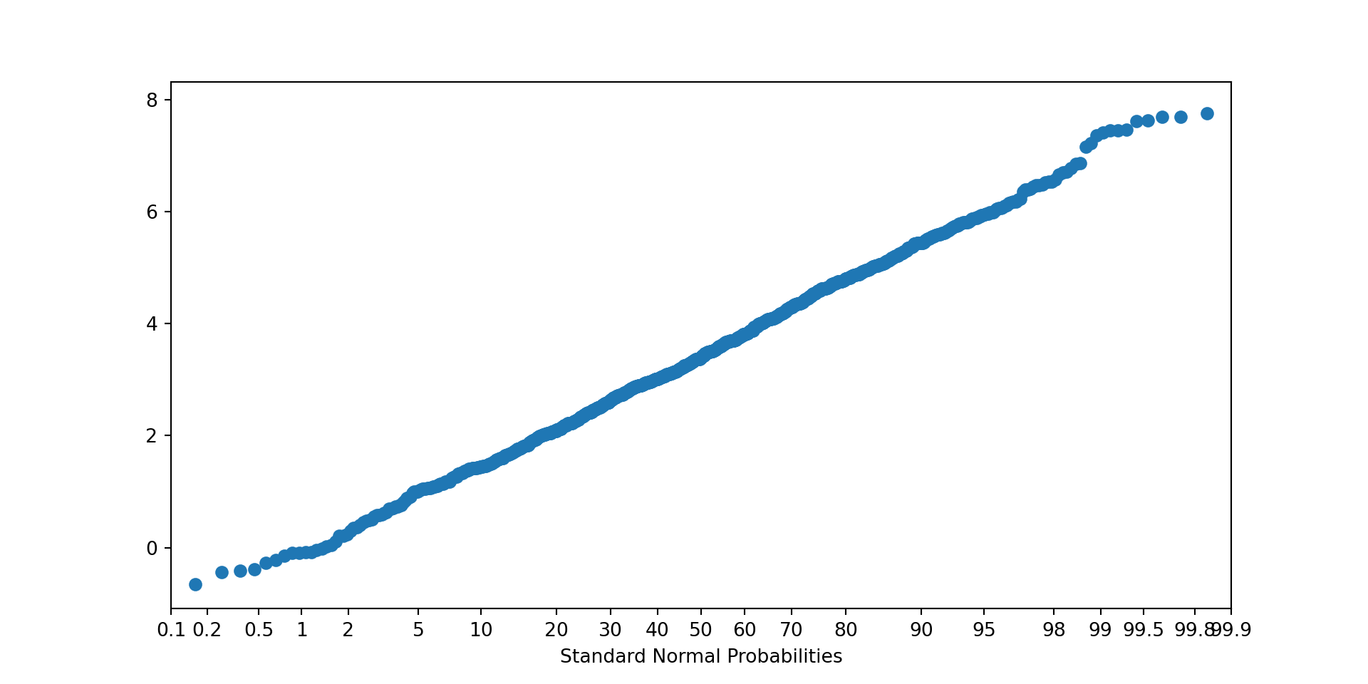
10:78 - MVJ
c.: We compute
Code
bs_margin = scipy.stats.norm.isf(.025)*np.std(bs_samples)
ci_bs_lo = scores.query("group=='E'").score.mean() - scores.query("group=='C'").score.mean() - bs_margin
ci_bs_hi = scores.query("group=='E'").score.mean() - scores.query("group=='C'").score.mean() + bs_margin

print(f"""
$\\sigma_{{bs}}$ | CI low | CI high
-|-|-
{np.std(bs_samples):.2f} | {ci_bs_lo:.2f} | {ci_bs_hi:.2f}
""")| \(\sigma_{bs}\) | CI low | CI high |
|---|---|---|
| 1.55 | 0.44 | 6.50 |
10:78 - MVJ
d.: We need the percentiles from the bootstrap sample. Numpy provides:
Code
| 2.5% | 97.5% |
|---|---|
| 0.47 | 6.47 |
10:78 - MVJ
e.: Our CIs are:
Code
| Type | Low | High |
|---|---|---|
| Z-method | 0.29 | 6.64 |
| Bootstrap Std.Error | 0.44 | 6.50 |
| Bootstrap Quantiles | 0.47 | 6.47 |
Using the normal distribution and the z-method does not perform all that badly - with this large a data sample, the central limit theorem kicks in to validate using the normal distribution even if the distributions are not themselves normal.
f.: Do these results agree with Example 10.4?
Example 10.4 found a p-value of 0.016 for the two independent samples z-test and rejected the null hypothesis. In all our confidence intervals, 0 is not included in the CI, which corresponds to rejecting a two-tailed test.
10:79 - Justin Ramirez
a.: If a permutation test is done with 5000 arrangements (4999) random arrangements:
comparing the mean differences between the original and the observations: \(\overline x-\overline y=27.34118-23.87342 =- 3.467759\) given in a table in the book.
4921 of the 5000 of the permutations are less than or equal to the sample mean difference so the corresponding p-value is 0.0158 and after we double it, it is 0.0316 which means the null hypothesis is rejected.
b.: Due to the large sample sized, and the normality of the assumptions made in the test the two results are the same. If this was not the case then the null hypothesis would not be rejected.
10:80 - Justin Ramirez
Using the following code in Python:
The median of the control is 28 and the median of the experimental is 29. Based on the stem-leaf graph the reason the medians are similar is because of the extreme values/outliers presented in the data.
b.:
There are 85 data entries for the experimental group and 79 for the control. If 5000 different permutations of the data are taken:
we can compare the difference between the first 85 observations and the remaining ones. The mean difference of the original sample is 29-28 = 1.
Of the 5000 permutation differences, there are 2878 that are smaller than or equal to the sample mean difference, and this means there is a p-value of 0.422 which means the null hypothesis is rejected.
Note on Permutation Tests
To perform a permutation test, we can use the same .sample(frac=1.0) from pandas that we have been using for bootstraps, only this time sampling without replacement. Sampling the entire dataset randomly without replacement will just shuffle the entries.
So the permutation test Justin describes can be performed as follows:
Code
perm_samples = [perm[:85].median() - perm[85:].median() for _ in range(4999) for perm in [scores.score.sample(frac=1.0, replace=False)]]
print(f"""
$\\#\\{{perm < 1\\}}$ | p-value | unbiased p-value
-|-|-
{(np.array(perm_samples) < 1.0).sum()} | {(np.array(perm_samples) < 1.0).sum()/len(perm_samples):.2f} | {((np.array(perm_samples) < 1.0).sum()+1)/(len(perm_samples)+1):.2f}
""")| \(\#\{perm < 1\}\) | p-value | unbiased p-value |
|---|---|---|
| 2846 | 0.57 | 0.57 |