ANOVA

Mikael Vejdemo-Johansson

\[ \def\RR{{\mathbb{R}}} \def\PP{{\mathbb{P}}} \def\EE{{\mathbb{E}}} \def\VV{{\mathbb{V}}} \]

One mean, Two means, Many means

Many of our tests have focused on comparing means of groups:

Null Hypothesis Type	Test Type
\(H_0:\mu = \mu_0\)	One-sample T test
\(H_0:\mu_1 = \mu_2\)	Two-sample T test

We will next introduce the next step in this progression: comparing means for more than 2 subgroups of a set of observations.

Our setup thus is going to be that we have some collection of samples, each from a separate normal distribution, with the same variance for each sample. We will be interested in testing:

\(H_0:\mu_1 = \dots = \mu_I\) vs. the alternative that at least one pair of groups have different means.

Notation and Assumptions

For this, we will use the following notation:

• \(X_{1,1},\dots,X_{I,J}\) are our observed random variables.
• \(X_{i,1},\dots,X_{i,J}\sim\mathcal{N}(\mu_i, \sigma^2)\).
• \(\overline{X}_{i,*} = \frac{1}{J}\sum_{j=1}^J X_{i,j}\), the group-wise sample means.
• \(\overline{X}_{*,*} = \frac{1}{IJ}\sum_{i=1}^I\sum_{j=1}^J X_{i,j}\), the grand sample mean.
• \(S_1^2,\dots,S_I^2\) are the sample variances of the groups \(1\) through \(I\).

Upper-case letters will denote random variables (or total sizes, for \(I\) and \(J\)), and lower-case letters are observations or realizations of those random variables.

Checking the assumptions

We have two important assumptions that we are making:

1. Each observation is normal.
2. All variances are equal.

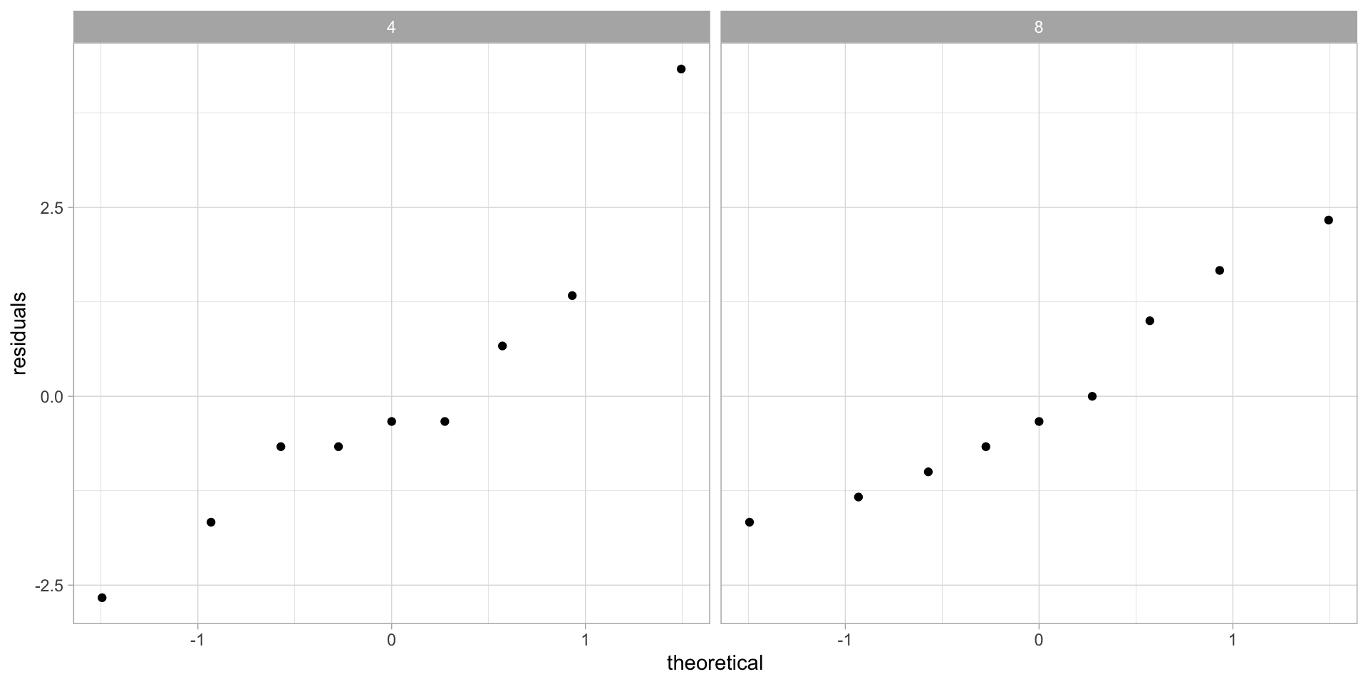
To check 1., we could use individual probability plots for each group. Alternatively, we can compute the residuals \(r_{i,j} = x_{i,j}-\overline{x}_{i,*}\), and check that all the residuals taken as one group form a normal distribution.

Running Example

Autistic and Neurotypical Peer-to-peer Information Sharing

CJ Crompton, D Ropar, CVM Evans-Williams, EG Flynn, S Fletcher-Watson, Autistic peer-to-peer information transfer is highly effective, Autism (2020) 24:7, doi:10.1177/1362361320919286

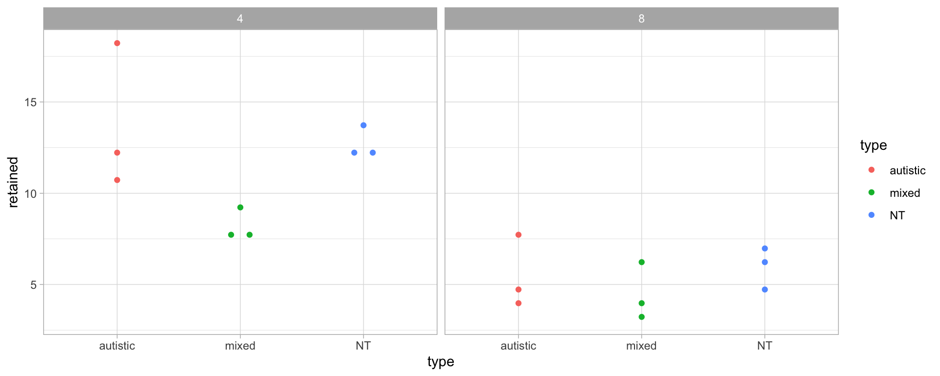
The research project recruited 9 groups of 8 participants to form “game of telephone” communication chains. 3 chains were only with autistic adults. 3 chains were only with neurotypical adults. 3 chains were alternating NT-autistic-NT-autistic-NT-autistic-NT-autistic. First person in each chain was told a complex and bizarre story by the researchers, and then each person in the chain re-told the story to the next person in the chain. At each step, they measured how many of the story details were retained.

After everything, they also measured by a self-reporting survey, their feelings of ease, enjoyment, success, friendliness, awkwardness.

Running Example

Autistic and Neurotypical Peer-to-peer Information Sharing

The number of retained story details (out of a total of 30) after each step were:

Code

story.chains = tribble(
    ~step, ~chain1, ~chain2, ~chain3, ~chain4, ~chain5, ~chain6, ~chain7, ~chain8, ~chain9,
    1,25,20,19,23,15,15,24,19,18,
    2,19,16,16,12,13, 9,20,18,16,
    3,17,15,14,10,10, 9,19,13,13,
    4,14,12,12, 8, 9, 8,18,12,11,
    5,11,12, 9, 8, 7, 8,15,11,10,
    6, 7, 9,10, 7, 5, 8,13,10, 8,
    7, 7, 9, 6, 6, 4, 7, 8, 9, 7,
    8, 6, 5, 7, 4, 3, 6, 8, 4, 5,
)
chain.type = tibble(
  chain=paste0("chain", 1:9),
  type =rep(c("NT", "mixed", "autistic"), each=3)
)
story.chains %>% kable %>% kable_styling(bootstrap_options = "condensed", font_size=16)
chain.type %>% t %>% kable %>% kable_styling(bootstrap_options = "condensed", font_size=16)

step	chain1	chain2	chain3	chain4	chain5	chain6	chain7	chain8	chain9
1	25	20	19	23	15	15	24	19	18
2	19	16	16	12	13	9	20	18	16
3	17	15	14	10	10	9	19	13	13
4	14	12	12	8	9	8	18	12	11
5	11	12	9	8	7	8	15	11	10
6	7	9	10	7	5	8	13	10	8
7	7	9	6	6	4	7	8	9	7
8	6	5	7	4	3	6	8	4	5

chain	chain1	chain2	chain3	chain4	chain5	chain6	chain7	chain8	chain9
type	NT	NT	NT	mixed	mixed	mixed	autistic	autistic	autistic

Running Example

Autistic and Neurotypical Peer-to-peer Information Sharing

I claim that after 4 retellings, there is a significant difference among these three group, but after 8 retellings, they are very similar again.

We could choose to study how many story details made it intact through 8 retellings. This would give us the following data set split into groups:

Code

library(ggbeeswarm)
story.last = story.chains[c(4,8),] %>%
  pivot_longer(starts_with("chain"), names_to="chain", values_to="retained") %>%
  inner_join(chain.type, by="chain")
story.last.summaries = story.last %>% 
  group_by(step, type) %>% summarise(m=mean(retained), s=sd(retained))
ggplot(story.last, aes(x=type, y=retained, color=type)) +
  geom_beeswarm(method="center", cex=5) +
  facet_grid(~step)

Running Example

Autistic and Neurotypical Peer-to-peer Information Sharing

In the notation we have established, we have:

step	\(I\)	\(J\)	\(\overline{X}_{1,*}\)	\(\overline{X}_{2,*}\)	\(\overline{X}_{3,*}\)	\(\overline{X}_{*,*}\)	\(S_1^2\)	\(S_2^2\)	\(S_3^2\)
4	3	3	12.7	8.3	13.7	11.6	1.2	0.6	3.8
8	3	3	6	4.3	5.7	5.3	1	1.5	2.1

Running Example

Autistic and Neurotypical Peer-to-peer Information Sharing

For a normality check, we would subtract group means from each observation to get the corresponding residuals.

Code

story.residuals = story.last %>% group_by(step, type) %>%
  mutate(residuals=retained-mean(retained))
ggplot(story.residuals, aes(sample=residuals)) +
  geom_qq() +
  labs(y="residuals") +
  facet_grid(~step)

ANOVA - basic idea

The basic approach of the ANOVA is to separate out the variance observed in the sample into portions contributed by different sources.

Code

library(patchwork)

df = tibble(
  x = rnorm(50),
  y = rnorm(50),
  z = rnorm(50),
  w = rnorm(50, 2.0)
) %>% pivot_longer(everything())
d1w = ggplot(df, aes(x=value)) +
  geom_density(data=function(r) r %>% filter(name != "w")) +
  labs(title=str_glue("std = {round(sd((df %>% filter(name != 'w'))$value), 2)}"))
daw = ggplot(df, aes(x=value)) +
  geom_density(aes(color=name), data=function(r) r %>% filter(name != "w"))
d1z = ggplot(df, aes(x=value)) +
  geom_density(data=function(r) r %>% filter(name != "z")) +
  labs(title=str_glue("std = {round(sd((df %>% filter(name != 'z'))$value), 2)}"))
daz = ggplot(df, aes(x=value)) +
  geom_density(aes(color=name), data=function(r) r %>% filter(name != "z"))

((d1w | daw)/(d1z | daz)) & (
  xlim(-6,6)
)

ANOVA - Fundamental Identity

Definition

Total Sum of Squares

\(SST = \sum_i\sum_j(X_{i,j}-\overline{X}_{*,*})^2\)

Treatment Sum of Squares

\(SSTr = \sum_i\sum_j(\overline{X}_{i,*}-\overline{X}_{*,*})^2\)

\(\phantom{SStr = }J\sum_i(\overline{X}_{i,*}-\overline{X}_{*,*})^2\)

Error Sum of Squares

\(SSE = \sum_i\sum_j(X_{i,j}-\overline{X}_{i,*})^2\)

Fundamental Identity of ANOVA

\(SST = SSTr + SSE\)

ANOVA - Fundamental Identity

Fundamental Identity of ANOVA

\(SST = SSTr + SSE\)

Proof

\[ \begin{align*} x_{i,j}-\overline{x}_{*,*} &= x_{i,j}+(-\overline{x}_{i,*}+\overline{x}_{i,*}) - \overline{x}_{*,*}) \\ &= (x_{i,j}-\overline{x}_{i,*})+(\overline{x}_{i,*} - \overline{x}_{*,*}) & \text{square both sides}\\ (x_{i,j}-\overline{x}_{*,*})^2 &= \left(\color{Teal}{(x_{i,j}-\overline{x}_{i,*})}+\color{DarkMagenta}{(\overline{x}_{i,*} - \overline{x}_{*,*})}\right)^2 \\ &= \color{Teal}{(x_{i,j}-\overline{x}_{i,*})}^2 + 2\color{Teal}{(x_{i,j}-\overline{x}_{i,*})}\color{DarkMagenta}{(\overline{x}_{i,*} - \overline{x}_{*,*})} + \color{DarkMagenta}{(\overline{x}_{i,*} - \overline{x}_{*,*})}^2 & \text{sum over all }i,j \\ SST = \sum_i\sum_j(x_{i,j}-\overline{x}_{*,*})^2 &= \underbrace{\sum_i\sum_j(x_{i,j}-\overline{x}_{i,*})^2}_{=SSE} + 2\sum_i(\overline{x}_{i,*}-\overline{x}_{*,*})\sum_j(x_{i,j}-\overline{x}_{i,*}) + \\ &\phantom{= } \underbrace{\sum_i\sum_j(\overline{x}_{i,*} - \overline{x}_{*,*})}_{=SSTr} \\ \sum_j(x_{i,j}-\overline{x}_{i,*}) &= 0 \end{align*} \]

Degrees of Freedom

SST has \(IJ-1\) degrees of freedom

There are \(IJ\) terms in the sum that defines the SST, but they all include the term \(\overline{x}_{*,*}\), so there is one connecting equation for all of them.

SSE has \(I(J-1)\) degrees of freedom

There are \(IJ\) terms in the sum that defines the SSE, but there are \(I\) different group means, each of which defines a connecting equation, so the total degrees of freedom comes out to \(IJ-I = I(J-1)\).

SSTr has \(I-1\) degrees of freedom

There are \(I\) distinct variables \(\overline{x}_{i,*}\) in the sum that defines the SSTr, but the \(\overline{x}_{*,*}\) connects all of them in a connecting equation.

Variance Estimates

All three sum of squares can be used to estimate \(\sigma^2\) - the variance that according to our assumptions all the data sources share:

Definition

\[ MST = \frac{SST}{IJ-1}\qquad MSE = \frac{SSE}{I(J-1)}\qquad MSTr = \frac{SSTr}{I-1} \]

Theorem

\[ \EE[MSE] = \sigma^2 \]

Additionally, if \(H_0\) is true, then \[ \EE[MST] = \sigma^2 \qquad \EE[MSTr] = \sigma^2 \]

Variance Ratios

From this follows that under the null hypothesis,

\[ \begin{align*} \frac{MSE}{\sigma^2} = \frac{SSE/(I(J-1))}{\sigma^2} &\sim \chi^2(I(J-1)) \\ \frac{MST}{\sigma^2} = \frac{SST/(IJ-1)}{\sigma^2} &\sim \chi^2(IJ-1) \\ \frac{MSTr}{\sigma^2} = \frac{SSTr/(I-1)}{\sigma^2} &\sim \chi^2(I-1) \\ \frac{MSTr/\sigma^2}{MSE/\sigma^2} = \frac{MSTr}{MSE} &\sim F(I-1,I(J-1)) \end{align*} \]

If the null hypothesis is false, then (in your homework you will) show that \(MSTr\) is larger than expected, so the ratio is larger and we can reject the null hypothesis with the upper tail of the \(F\) distribution.

The One-way ANOVA Test

One-way Analysis of Variance

Null Hypothesis

\(H_0:\mu_1=\dots=\mu_I\)

Test Statistic

\(F = \frac{MSTr}{MSE}\)

Rejection Region for Level \(\alpha\)

\(F > CDF_{F(I-1,I(J-1))}^{-1}(1-\alpha)\)

p-value

\(1-CDF_{F(I-1,I(J-1))}(F)\)

Running Example

Autistic and Neurotypical Peer-to-peer Information Sharing

We have established that the data seems to have normal errors (both after 4 steps and after 8 steps). Recall that we had:

step	\(I\)	\(J\)	\(\overline{X}_{1,*}\)	\(\overline{X}_{2,*}\)	\(\overline{X}_{3,*}\)	\(\overline{X}_{*,*}\)	\(S_1^2\)	\(S_2^2\)	\(S_3^2\)
4	3	3	12.7	8.3	13.7	11.6	1.2	0.6	3.8
8	3	3	6	4.3	5.7	5.3	1	1.5	2.1

For the one-way ANOVA test, we need to compute the entries in an ANOVA Table

Code

SSE = story.residuals %>% group_by(step) %>%
  summarise(SSE=sum(residuals^2))
SSTr = story.last.summaries %>%
  group_by(step) %>%
  summarise(SSTr=sum((m-mean(m))^2)*(length(m)-1))
SST = story.last %>% group_by(step) %>%
  summarise(SST=sum((retained-mean(retained))^2))
SS = list(SSE, SSTr, SST) %>% 
  reduce(left_join, by="step") %>%
  mutate(MSE=SSE/(3*2), MSTr=SSTr/2, MST=SST/(3*3-1)) %>%
  mutate(F=MSTr/MSE, p=pf(F, 2, 6, lower.tail=FALSE))

Step 4

Source	SS*	DoF	MS*	F	p
Treat.	32.15	2	16.07	3.01	0.12
Error	32	6	5.33
Total	80.22	8	10.03

Step 8

Source	SS*	DoF	MS*	F	p
Treat.	3.11	2	1.56	0.61	0.57
Error	15.33	6	2.56
Total	20	8	2.5

Formally Testing for Equal Variances

The book recommends the Levene Test for testing for equal variances. This test is less sensitive than the Bartlett Test (which is what emerges from the likelihood ratio principle), and is done by running through a one-way ANOVA on the absolute values of the residuals.

Running Example, Equal Variances

Code

story.residuals %>% filter(step==4) %>%
  ungroup() %>%
  mutate(abs.residuals=round(abs(residuals),2)) %>%
  select(type, abs.residuals) %>%
  t %>% kable()
story.residuals %>% filter(step==8) %>%
  ungroup() %>%
  mutate(abs.residuals=round(abs(residuals),2)) %>%
  select(type, abs.residuals) %>%
  t %>% kable()

type	NT	NT	NT	mixed	mixed	mixed	autistic	autistic	autistic
abs.residuals	1.33	0.67	0.67	0.33	0.67	0.33	4.33	1.67	2.67

type	NT	NT	NT	mixed	mixed	mixed	autistic	autistic	autistic
abs.residuals	0.00	1.00	1.00	0.33	1.33	1.67	2.33	1.67	0.67

Running Example, Equal Variances

Step 4

Code

story.levene = story.residuals %>%
  filter(step == 4) %>%
  mutate(abs.residuals=abs(residuals), 
         chain.type=fct(type)) %>%
  ungroup() %>%
  select(chain.type, abs.residuals)
story.levene.aov = aov(abs.residuals ~ chain.type, story.levene)
anova(story.levene.aov)

Analysis of Variance Table

Response: abs.residuals
           Df Sum Sq Mean Sq F value  Pr(>F)  
chain.type  2 10.173  5.0864  7.6296 0.02248 *
Residuals   6  4.000  0.6667                  
---
Signif. codes:  0 '***' 0.001 '**' 0.01 '*' 0.05 '.' 0.1 ' ' 1

There may be a reason to doubt the equal variances assumption.

Step 8

Code

story.levene = story.residuals %>%
  filter(step == 8) %>%
  mutate(abs.residuals=abs(residuals), 
         chain.type=fct(type)) %>%
  ungroup() %>%
  select(chain.type, abs.residuals)
story.levene.aov = aov(abs.residuals ~ chain.type, story.levene)
anova(story.levene.aov)

Analysis of Variance Table

Response: abs.residuals
           Df Sum Sq Mean Sq F value Pr(>F)
chain.type  2 1.1852 0.59259  1.1707 0.3722
Residuals   6 3.0370 0.50617               

At the end, there seems to be less reason to doubt the equal variances assumption.

ANOVA as a modeling equation

There is a succinct way to describe the one-way ANOVA with a model equation:

\[ X_{i,j} = \mu_i + \epsilon_{i,j} \qquad \epsilon_{i,j}\sim\mathcal{N}(0,\sigma^2) \]

This model equation can be rewritten by introducing \(\mu=\frac{1}{I}\sum_i \mu_i\), and modeling the deviations from the global mean as parameters \(\alpha_1,\dots,\alpha_I\). Then, with \(I+1\) parameters, that are connected by one equation we still have \(I\) independently determined parameters and get the model equation

\[ X_{i,j} = \mu+\alpha_i+\epsilon_{i,j} \qquad \epsilon_{i,j}\sim\mathcal{N}(0,\sigma^2) \]

A new null hypothesis then becomes \(\alpha_1=\alpha_2=\dots=\alpha_I=0\).

ANOVA as a linear model

Suppose now that we represent membership in group \(i\) by the \(i\)th unit vector, so that we can represent e.g. the running example data (seen to the left) by a matrix like the one on the right instead:

Code

story.last %>% filter(step==4) %>%
  ungroup() %>% select(retained, type) %>%
  kable(caption="Values-Factor") %>%
  kable_styling(bootstrap_options = "condensed")
story.last %>% filter(step==4) %>%
  ungroup() %>% select(chain, type, retained) %>%
  mutate(value=1) %>% pivot_wider(names_from=type, values_from=value, values_fill=0) %>% select(-chain) %>%
  kable(caption="One-Hot encoded Factors") %>%
  kable_styling(bootstrap_options = "condensed")

Values-Factor

retained	type
14	NT
12	NT
12	NT
8	mixed
9	mixed
8	mixed
18	autistic
12	autistic
11	autistic

One-Hot encoded Factors

retained	NT	mixed	autistic
14	1	0	0
12	1	0	0
12	1	0	0
8	0	1	0
9	0	1	0
8	0	1	0
18	0	0	1
12	0	0	1
11	0	0	1

ANOVA as a linear model

With this one-hot encoding, we can represent the modeling equation as a linear equation with somewhat restricted predictor variables:

\[ X_{i,j} = \mu + \sum_{i\in I}\alpha_i\cdot \beta_{i,j} + \epsilon_{i,j} \]

where the \(\beta_{i,j}\) are the one-hot encoded variables, so at most one of these \(\beta_{i,j}\) is non-zero (and therefore \(=1\)) at any given point.

Modeling Formulas

This specification of the ANOVA model using predictor variables and response variables is of core importance for using computational software¹ to compute for us.

In R, it is a very common convention to write “\(Y\) is predicted by \(X\)” as Y ~ X (and if we expect \(Y=\beta_1 X_1+\beta_2 X_2\) we would write something like Y ~ X.1 + X.2)

1. …or at least for using R

ANOVA automated commands

In R

In R, ANOVAs are handled very similar to linear regression computations. Counter-intuitively, the command anova does not run an ANOVA model, but instead outputs the ANOVA table for a large class of possible models. Instead, the aov command runs a linear model with the expectation that it be an ANOVA model.

To use aov, first make sure that your data is in long shape - that is to say, values of interest in one column (say retained for the running example) and group membership in another column (say type for the running example).

Then an ANOVA analysis is performed by the aov command, which by default outputs the response as a truncated ANOVA table. To get a full ANOVA table, use the anova command on its output:

Code

model = aov(retained ~ type, story.last %>% filter(step==4))
anova(model)

Analysis of Variance Table

Response: retained
          Df Sum Sq Mean Sq F value  Pr(>F)  
type       2 48.222 24.1111  4.5208 0.06347 .
Residuals  6 32.000  5.3333                  
---
Signif. codes:  0 '***' 0.001 '**' 0.01 '*' 0.05 '.' 0.1 ' ' 1

ANOVA automated commands

In Python

SciPy provides the command scipy.stats.f_oneway for performing one-way ANOVA tests. Each separate group is given as a separate argument for the function.

Code

NT = [14, 12, 12]
mixed = [8, 9, 8]
autistic = [18, 12, 11]
scipy.stats.f_oneway(NT, mixed, autistic)

F_onewayResult(statistic=4.52083333333333, pvalue=0.06346961596914304)