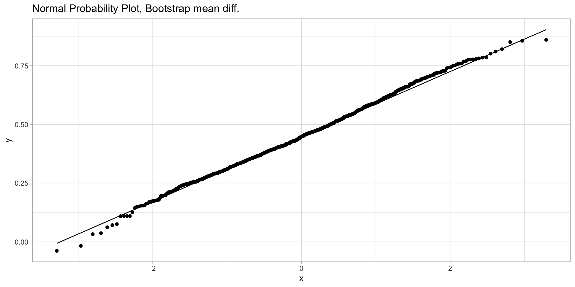
To use the bootstrap for two samples we follow very similar procedures to the ones for the one-sample bootstrap. The main difference is that we take simultaneous and separate samples with replacement from both groups. With the samples, compute some statistic to compare them, repeat for a large number of times.
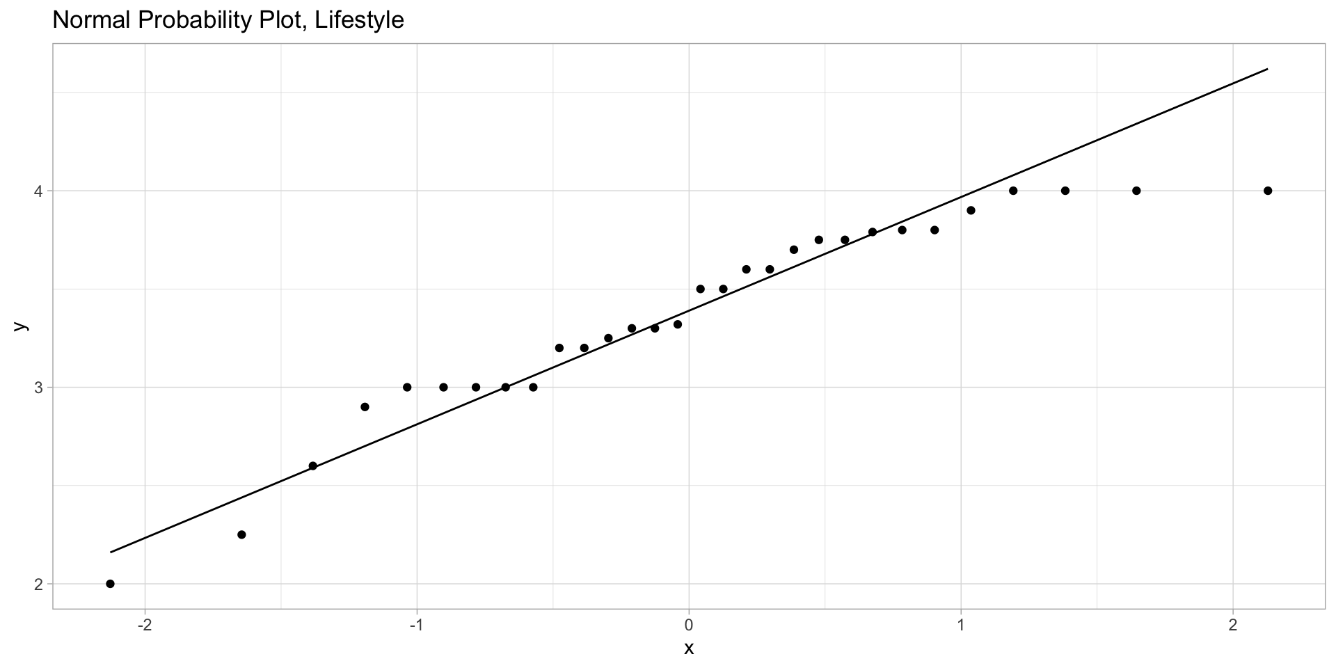
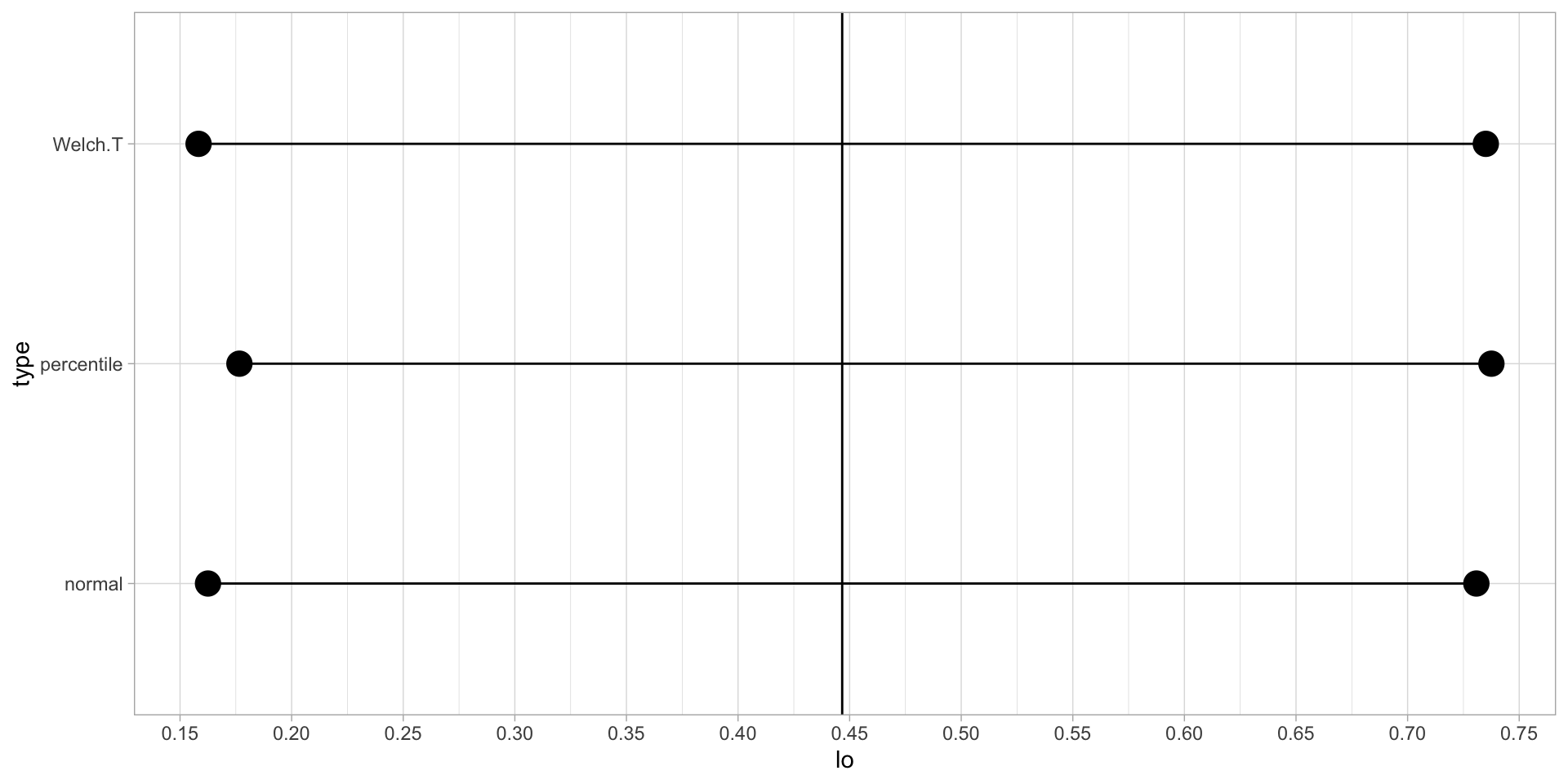
If the resulting statistics seem normally distributed, we can use the normal bootstrap confidence intervals - if not, we should use the basic, or the percentile, or the studentized method - where for the studentized method we would collect \(t\)-values and find quantiles of those.
Two-Sample Bootstrap; Exercise 10.69
We are given GPA scores from 30 students on so-called lifestyle floors in a dorm, and from 30 students on other floors:
If we reduce the degrees of freedom, the T-distribution gets fatter tails, so higher probability for more extreme outcomes, which makes the p-values larger and the CI wider.
It is a “safe” change, because choosing our degrees of freedom too low is conservative (ie, will give us a lower actual significance level or higher confidence level than we actually try to get) and our probability of false rejections is lower than we try to get it.
Chapter 10; Exercise 110
We are picking up McNemar’s test again, from last lecture. We are given pairs of individuals, each treated with either Ergotamine or Placebo for migraine headaches, and the following (fictitous) data:
Ergotamine
S
F
Placebo
S
44
34
F
46
30
McNemar’s test statistic uses the SF and FS combined counts: \[
Z=\frac{46-34}{\sqrt{46+34}} \approx 1.341641 \\
p = 1-\Phi(1.341641) \approx 0.08985625
\]
An upper-tail McNemar test does not support rejecting the null hypothesis at \(\alpha=0.05\). Ergotamine does not seem significantly more effective than placebo.
Chapter 10; Exercise 111
Let \(X_1,\dots,X_{n_X}\sim Poisson(\lambda_X)\) iid and independently \(Y_1,\dots,Y_{n_Y}\sim Poisson(\lambda_Y)\) iid.
From \(\VV[\overline{P}]=\lambda/n\) for Poisson distributed samples \(P_i\) and from the independence of the samples follows that \(\VV[\overline{X}-\overline{Y}] = \frac{\lambda_X}{n_X} + \frac{\lambda_Y}{n_Y}\).
Combining these we get a test statistic with a standard normal distribution under \(H_0\): \[
Z=\frac{\overline{X}-\overline{Y}}{\sqrt{\frac{\overline{X}}{n_X}+\frac{\overline{Y}}{n_Y}}}
\]
one test for \(H_{01}:\theta\in\Omega_1\) vs. \(H_{a1}:\theta\not\in\Omega_1\) with rejection region \(R_1\) at significance level \(\alpha\),
another test for \(H_{02}:\theta\in\Omega_2\) vs. \(H_{a2}:\theta\not\in\Omega_2\) with rejection region \(R_2\) at significance level \(\alpha\)
And that \(\Omega_1\) and \(\Omega_2\) are disjoint sets of possible values for the parameter \(\theta\).
We have a proposed test (the Union-Intersection Test) for \(H_0:\theta\in\Omega_1\cup\Omega_2\) vs. \(H_a:\theta\not\in\Omega_1\cup\Omega_2\) with proposed rejection region \(R_1\cap R_2\).
Where the inequalities are because we are expanding the event in each case.
Chapter 10; Exercise 113
b. Let \(\mu_T\) be the mean value of some variable for a generic (test) drug, and \(\mu_R\) the same for a brand-name (reference) drug. Bioequivalence testing would test \(H_0:\mu_T/\mu_R\leq\delta_L\) or \(\mu_T/\mu_R\geq\delta_U\) versus \(H_a:\delta_L<\mu_T/\mu_R <\delta_U\) (bioequivalence), where \(\delta_L\) and \(\delta_U\) are standards set by regulatory agencies - FDA uses 0.80 and 1.25=1/0.80 for certain cases, and mandates \(\alpha=0.05\).
Take logarithms, and the question becomes one of testing for differences rather than ratios.
Let \(D\) be an estimator of \(\log\mu_T-\log\mu_R\) with standard error \(S_D\). The standardized variable \(T = \frac{D-(\log\mu_T-\log\mu_R)}{S_D}\sim T(\nu)\). The standard test procedure in this setup is the TOST - two one-sided tests, and uses the two test statistics \(T_U=(D-\log\delta_U)/S_D\) and \(T_L=(D-\log\delta_L)/S_D\).
Concrete examples
Using \(\nu=20\) degrees of freedom and a one-sided cut-off \(t_{0.05,20}\approx1.724\), we get the following outcomes:
Case 1
Case 2
Case 3
\(T_L\)
2.0
1.5
2.0
\(T_U\)
-1.5
-2.0
-2.0
Reject \(L\)
Yes
No
Yes
Reject \(U\)
No
Yes
Yes
Reject \(H_0\)
No
No
Yes
Your Homework
10:14 - Justin Ramirez
The z-score for \(\theta\) is1\[
z = \frac{\hat\theta-\theta_0}{\sigma_\theta}
\]
The Null Hypothesis is: \(H_0: \theta-\theta_0=0\).
The alternative hypothesis is: \(H_1:\theta-\theta_0\neq 0\)
Since we are given the parameter: \(\theta=2\mu_1-\mu_2\) which means \(\hat\theta=2\overline{X}_1-\overline{X}_2\)
To find the standard deviation: Expected value of \(\hat\theta: \theta=2\mu_1-\mu_2\)
The variance is: \[
\VV=\VV(2\overline{X}_1-\overline{X}_2) \Rightarrow
4\VV(\overline{X}_1)+\VV(\overline{X_2}) \Rightarrow
4\left(\frac{\sigma_1^2}{n_1}\right)+\left(\frac{\sigma_2^2}{n_2}\right)
\]
So the standard error is: \(\sigma_{\hat\theta}=\sqrt{4\left(\frac{\sigma_1^2}{n_1}\right)+\left(\frac{\sigma_2^2}{n_2}\right)}\)
So to get the z-score: \[
z = \frac{(2\overline{X}_1-\overline{X}_2)-(2\mu_1-\mu_2)}{\sqrt{4\left(\frac{\sigma_1^2}{n_1}\right)+\left(\frac{\sigma_2^2}{n_2}\right)}}
\]
Plug in: A test done at 0.01 shows:
\[
z = \frac{2\cdot 2.69 - 6.35}{\sqrt{4\left(\frac{2.3^2}{43}\right)+\left(\frac{4.03^2}{45}\right)}}
\approx -1.050259774
\] which shows that at 0.1 it fails to reject the Null hypothesis.
The standard deviation is: \(\sigma=\sqrt{\frac{\sum(d_i-\overline{d})^2}{n-1}}\Rightarrow\sqrt{\frac{4.787}{32}}\approx 0.38677\)
The degrees of freedom is equal to \(n-1\), so 32.
The level of significance is \(\alpha=0.05\).
Using the t table at 0.05 with 32 degrees of freedom: \(t_{\alpha/2}=\pm2.037\)
To get the CI: \[
-0.42394\pm2.037\cdot\left(\frac{0.38677}{\sqrt{33}}\right) \Rightarrow
-0.42394\pm0.13714\Rightarrow(-0.561, -0.287)
\]
10:40 b. - Justin Ramirez
The prediction interval for the 34th house would be: \[
\overline{z}\pm t_{0.025,32}\cdot\sigma\sqrt{1+\frac{1}{n}} \\
\Rightarrow-0.42394\pm2.037\cdot0.38677\sqrt{1+\frac{1}{33}} \\
\Rightarrow-0.42394\pm0.799699 \\
\Rightarrow\boxed{(-1.224,0.376)}
\]