Two-sample Inference: Paired Data
\[ \def\RR{{\mathbb{R}}} \def\PP{{\mathbb{P}}} \def\EE{{\mathbb{E}}} \def\VV{{\mathbb{V}}} \]
Paired Samples
Our ability for counter-factual causal analysis improves if we can make two different measurements on the same unit, rather than comparing measurements made in different part of the population.
These sort of paired measurements can be made in a variety of different situations:
- studies on twins, where each twin is subjected to a different treatment
- studies on parent/child pairs
- studies on locations, with repeated measurement at each location
- studies on the same individual, before and after some procedure or exposure
Fundamental to this sort of paired study design is that an assumption of independence between the two groups is no longer possible: something is connecting the paired units, producing a dependence between them. We crucially used this independence assumption in deriving the standard error for the denominator of the test statistic / pivot variable.
Because the independence issue, you cannot use standard two-sample methods on paired data (…unless you can verify that there is no correlation going on…); the distinction between paired and unpaired has to happen at the stage of experiment design, not at the stage of analyzing experimental data.
Choosing a paired design will bring your degrees of freedom down from around \(2n\) to around \(n\), producing lower precision, lower power, and a higher probability of false acceptances.
But we were also relying on randomization to remove bias in our argument for experiments enabling causal analyses. And so, if it is genuinely difficult to make the population split into homogenous treatment groups, a paired design would bring down variance dramatically, improving precision and power.
Paired or Unpaired
Choose Paired Experiments When…
There is great heterogeneity between experimental units, and large correlation within experimental units. The loss in degrees of freedom will be compensated by the decreased variance and incrased precision.
Choose Independent Samples Experiments When…
The experimental units are relatively homogenous, and the correlation within pairs is not large. The gain of precision from pairing will be outweighted by the decrease in degrees of freedom.
Paired Data Analysis
We assume that our data comes in independently selected pairs \((X_1,Y_1), \dots, (X_n,Y_n)\) with \(\EE(X_i)=\mu_1\) and \(\EE(Y_i)=\mu_2\).
Define \(D_1=X_1-Y_1, \dots, D_n=X_n-Y_n\), so that the variables \(D\) are the differences within pairs.
We assume in order to develop analysis procedures that \(D_i\sim\mathcal{N}(\mu_D, \sigma^2_D)\), with the same mean and variance across all the differences.
After this change in variables, from the pairs \(X,Y\) to the differences \(D\), we have transformed a two-sample question into a one-sample question and can use one-sample techniques for analysis. Assuming normally distributed differences, it is natural to turn to the one sample T-test and T confidence interval.
Paired T Test
- Pre-computation
- Given pairs \((X_i,Y_i)\) following an arbitrary distribution, but with normally distributed differences, compute \(D_i=X_i-Y_i\). Write \(\overline{d}\) and \(s_D\) for the sample mean and sample standard deviation of these observed differences \(d_i\).
- Null Hypothesis
- \(H_0:\mu_D = \Delta_0\), often chosen to be 0.
- Test Statistic
- \(t = \frac{\overline{d}-\Delta_0}{s_D/\sqrt{n}}\)
| Alternative Hypothesis | Rejection Region for Level \(\alpha\) | p-value | |
|---|---|---|---|
| Upper Tail | \(t>t_{\alpha,n-1}\) | \(1-CDF_{T(n-1)}(t)\) | |
| Two-tailed | \(|t|>t_{\alpha/2,n-1}\) | \(2\min\{CDF_{T(n-1)}(t), 1-CDF_{T(n-1)}(t)\}\) | |
| Lower Tail | \(t<-t_{\alpha,n-1}\) | \(CDF_{T(n-1)}(t)\) |
- Confidence Interval
- Upper bound: \(\mu_D < \overline{d} + t_{\alpha,n-1}s_D/\sqrt{n}\)
- Two-sided: \(\mu_D \in \overline{d}\pm t_{\alpha/2,n-1}s_D/\sqrt{n}\)
- Lower bound: \(\mu_D > \overline{d} - t_{\alpha,n-1}s_D/\sqrt{n}\)
Example 10.8
We are given zinc concentrations (mg/L) at six river locations at the surface and at the bottom.
Code
# Using Plotly for these plots
# pgo is the plotly.graph_objects module
fig = pgo.Figure(
  data=[\
    pgo.Scatter(x=[x for i in zinc.index for x in [i,i,None]],\
                y=[y for (s,b) in zip(zinc.surface, zinc.bottom) for y in [s, b, None]],\
                mode="lines", showlegend=False),
    pgo.Scatter(x=zinc.index, y=zinc.surface, mode="markers", name="surface"),
    pgo.Scatter(x=zinc.index, y=zinc.bottom, mode="markers", name="bottom")
  ]
)
#pgo.FigureWidget(fig)
fig.show()
Example 10.8
Verify that the differences seem normally distributed.
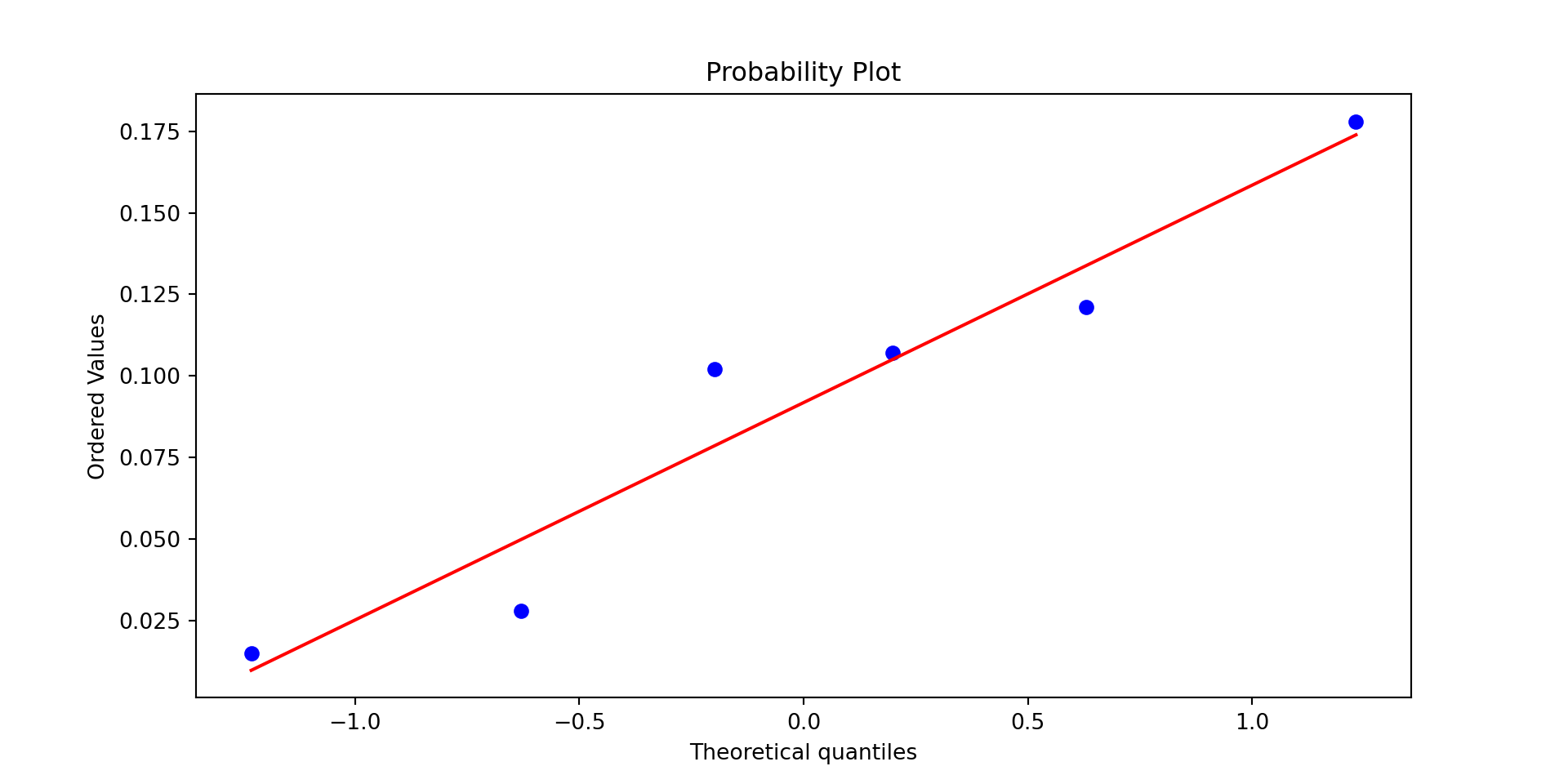
Example 10.8
Does the bottom concentration exceed the top concentration?
We compute:
Code
dbar = zinc.difference.mean()
se = zinc.difference.std()/len(zinc)
t = dbar/se
p = scipy.stats.t(len(zinc)-1).sf(t) # Upper tail test
t95 = scipy.stats.t(len(zinc)-1).ppf(0.95)
cb95 = dbar-t95*se

print(f"""
$\overline{{d}}$ | $S_D/\sqrt{{n}}$ | $T$ | df | $p$ | 95% lower CB
-|-|-|-|-|-
{dbar:.4f} | {se:.4f} | {t:.4f} | {len(zinc)-1} | {p:.4f} | {cb95:.4f}
""")| \(\overline{d}\) | \(S_D/\sqrt{n}\) | \(T\) | df | \(p\) | 95% lower CB |
|---|---|---|---|---|---|
| 0.0918 | 0.0102 | 9.0372 | 5 | 0.0001 | 0.0714 |
Pre-packaged T-test functionality
Both our software platforms provide for functions that will perform all the T-tests for us.
Python
scipy.stats.ttest_1samp(x, mu0)-
One-sample t-test of the data in
xagainst the population meanmu0. You may specifyalternative=the options"two-sided"(default),"less", or"greater". -
The return object has fields
statistic,pvalue,dfand a methodconfidence_interval(confidence_level=0.95). scipy.stats.ttest_ind(x, y, equal_var=True)-
Two independent samples t-test of the data in
xvs the data inyfor \(\Delta_0=0\). You may specifyalternativeas above. This assumes the pooled t-test, setequal_var=Falseto use Welch’s method instead. -
The return object has fields
statisticandpvalue. scipy.stats.ttest_ind_from_stats(mean1,std1,n1,mean2,std2,n2,equal_var=True)-
Two independent samples t-test from summary statistics instead of from data. You may specify
alternativeas above. This assumes the pooled t-test, setequal_var=Falseto use Welch’s method instead. -
The return object has fields
statisticandpvalue. scipy.stats.ttest_rel(x, y)-
Paired t-test of the data in
xvs the data inyfor \(\mu_D=0\). You may specifyalternativeas above. -
The return object has fields
statistic,pvalue,dfand a methodconfidence_interval(confidence_level=0.95).
Pre-packaged T-test functionality
Both our software platforms provide for functions that will perform all the T-tests for us.
R
t.test runs all our t-tests in one single function. Important generic arguments with their default values:
alternative="t"-
Takes values
"two.sided"(or"t"),"greater"(or"g"),"less"(or"l") mu=0- Your null-hypothesis \(\mu_0\) or \(\Delta_0\).
conf.level- Confidence level of the confidence interval that gets computed along with the test.
Depending on how you call the function, a different test is performed:
t.test(x)-
One-sample t-test of the data in
x. t.test(x,y)-
Two independent sample t-test with Welch’s method of
xvs.y. t.test(x,y, var.equal=TRUE)- Two independent sample t-test with equal variances.
t.test(x, y, paired=TRUE)- Paired t-test.
The test will print out a readable summary. If you assign a variable name (say test) to the test output, the object will have components test$statistic, test.parameter (df), p.value, conf.int, estimate (\(\overline{X}\) or \(\overline{X}-\overline{Y}\)), null.value, stderr (denominator of t-statistic), alternative, method
Chapter 10, Exercise 47
Construct a paired data set for which \(t=\infty\), so that the data is highly significant with the correct analyis, yet \(t\) for the two-sample test is quite near zero, so the incorrect analysis choice yields insignificant results.
To get to \(t=\infty\), the easiest way would be a division by zero. So if ALL differences in the data set were equal, that should do it.
To get the independent two-sample t-test small, we would like the two means to be very close to each other, so maybe if we took a bunch of sample points, and then shifted them all by something smaller than their spread.
Since the t-test functions don’t like division by zero, I added a tiny tiny bit of noise to my shift, just to get something out of both test functions.

Chapter 10, Exercise 47
Your Homework
9:40 - Victoria Paukova
\(H_0: p_0=.25\); \(H_a: p\neq.25\), \(\alpha=.01\), \(z=\frac{\hat p-p_0}{\sqrt{p_0(1-p_0)/n}}\)
Rejection region: \(Z \leq -2.58\) or \(Z \geq 2.58\) since \(Z_{\alpha/2} = 2.58\) and we want to use the two-tailed test.
\[ \hat p = \frac{177}{1050} \approx .16857; \quad z = \frac{.16857-.25}{\sqrt{.25\cdot.75/1050}} \approx -6.09 \]
The \(Z\) value is considerably out of the rejection region, so the data strongly argues for a conclusion of discrimination.
9:42 - Victoria Paukova
a.
We only reject \(H_0\) if the evidence points to a strong preference for gut strings, and \(H_0: p=.5\), \(np=10\). Out of the 3 rejection regions, the one that corresponds to the majority preferring gut strings (\(np>10\)) is \(\{15, 16, 17, 18, 19, 20\}\).
The other two regions are not appropriate because \(\{0,1,2,3,4,5\}\) means a small preference for gut strings, and \(\{0,1,2,3,17,18,19,20\}\) would be a two-tailed rejection region, which does not fit our case.
b.
\(\PP(X\geq 15) = 1-B(15-1; 20, .5) \approx .0207\). If we try again to get closer to .05, we can find \(\PP(X\geq 14) = 1-B(14-1; 20, .5)\approx 0.05765\). And trying again with \(c=16\) we get \(0.00591\), so the original region is the best level test.
MVJ: To hit exactly \(\alpha=0.05\), we would need a randomized test since the probability is discrete. An appropriate test function would be: \[ \phi(x) = \begin{cases} 1 & \text{if }x\geq15 \\ \gamma & \text{if }x=14 \\ 0 & \text{otherwise} \end{cases} \qquad \begin{align*} \EE[\phi(x)|H_0] &= \sum_{k=15}^{20} PMF_{Bin(20,.5)}(k) + \gamma\cdot PMF_{Bin(20,.5)}(14) = \alpha \\ \gamma &= \frac{\alpha - \sum_{k=15}^{20}PMF(k)}{PMF(14)} \approx \frac{0.05 - 0.0207}{0.037} \approx 0.793 \end{align*} \]
So if exactly 14 players preferred gut, we would draw a random number from \([0,1]\) and reject if it was below \(0.793\).
9:42 - Victoria Paukova
c.
\[ \begin{align*} \PP(X<15) = B(c-1; n, p') = B(14; 20, .6) &\approx .8744 \\ B(14; 20, .8) &\approx .19579 \end{align*} \]
d.
We reject \(H_0\) if 13 prefer gut strings at a .1 level. From the previous question, we already saw that the region starting at 14 would be the best .1 level test, so 13 is in the rejection region.
MVJ: Well, what we computed in b. was that \(X\geq 14\) would give us a level of .05765, we didn’t actually explore \(X=13\) there. Indeed, computing \(1-B(13-1; 20, .5) \approx 0.1316\), we see that including 13 in the rejection region gets us a level over .1.
But with a random test we might still reject \(H_0\) after seeing 13, since it is on the boundary. One test function we could use would be:
\[ \phi(x) = \begin{cases} 1 & \text{if }x\geq14 \\ \gamma & \text{if }x=13 \\ 0 & \text{otherwise} \end{cases} \qquad \begin{align*} \EE[\phi(x)|H_0] &= \sum_{k=14}^{20} PMF_{Bin(20,.5)}(k) + \gamma\cdot PMF_{Bin(20,.5)}(13) = \alpha \\ \gamma &= \frac{\alpha - \sum_{k=14}^{20}PMF(k)}{PMF(13)} \approx \frac{0.1 - 0.05765}{0.073929} \approx 0.573 \end{align*} \]
So a randomized test would reject \(57.3\%\) of the time.
9:55 - Victoria Paukova
\(H_0:\mu=3\); \(H_a:\mu\neq3\), a two-tailed test.
\(n=30, \overline{x}=2.481, s=1.616\), the hint tells us we can use the t-test distribution.
\[ t = \frac{\overline{x}-\mu_0}{s/\sqrt{n}} \approx -1.759;\qquad p = 2\PP(T>|t|) \approx 2\cdot 0.04456 \approx .08912 \]
Since our p-value of .08912 is less than .1, we have to reject \(H_0\).
With a sig level of .05, we would not reject H0, since .08912 is greater than .05.

9:66 - MVJ
Recall the CDFs and PDFs of the order statistics: \[ CDF_{X_{(1)}}(x) = 1-(1-CDF_X(x))^n \qquad\qquad PDF_{X_{(1)}}(x) = n(1-CDF_X(x))^{n-1}PDF_X(x) \]
If \(PDF_{X|\theta}(x) = e^{-(x-\theta)}\), then \[ \begin{align*} CDF_{X|\theta}(x) = \int_{\theta}^x PDF_{X|\theta}(y) dy &= \int_{\theta}^x e^{-(y-\theta)} dy \\ \text{substitute }u=\theta-y; du = -dy\qquad &= -\int_{0}^{\theta-x}e^{-u} du \\ &= -\left[e^{u}\right]_{0}^{\theta-x} \\ &= -(e^{-(x-\theta)}-1) = 1 - e^{-(x-\theta)} \\ \mathcal{LR}(x_{(1)}) &= \frac {n(1-CDF_{X|\theta_a}(x))^{n-1}PDF_{X|\theta_a}(x)} {n(1-CDF_{X|\theta_0}(x))^{n-1}PDF_{X|\theta_0}(x)} \\ &= \frac {\not n(1-(1-e^{-(x_{(1)}-\theta_a)}))^{n-1}e^{-(x_{(1)}-\theta_a)}} {\not n(1-(1-e^{-(x_{(1)}-\theta_0)}))^{n-1}e^{-(x_{(1)}-\theta_0)}} \\ &= e^{-n(x_{(1)}-\theta_a) - (-n(x_{(1)}-\theta_0))} \\ &= e^{n(x_{(1)}-\theta_0)-n(x_{(1)}-\theta_a)} = e^{n\theta_a-n\theta_0} \end{align*} \]
Except if \(\mathcal{L}(\theta_a) = 0\) and \(\mathcal{L}(\theta_0)\neq 0\). In those cases we get \(\mathcal{LR}=0\).
Hence, as a function of \(x_{(1)}\), the likelihood ratio is an increasing function, and hence has a rejection region \(\{x_{(1)} > c\}\) for some threshold value \(c\).
9:71 - MVJ
a. The setup is \(X_1,\dots,X_n\sim\mathcal{N}(\mu,\sigma^2)\), \(H_0:\mu=\mu_0\) vs. \(H_a:\mu\neq\mu_0\). In the example, the likelihood ratio is calculated to be:
\[ \begin{align*} \mathcal{LR} &=\left(\frac{\sum(x_i-\overline x)^2}{\sum(x_i-\mu_0)^2}\right)^{n/2} = \left(\frac{\sum((x_i-\overline{x})+(\overline{x}-\mu_0))^2}{\sum(x_i-\overline{x})^2}\right)^{-n/2} \\ &= \left(\frac{\sum(x_i-\overline{x})^2+2(\overline{x}-\mu_0)\sum(x_i-\overline{x}) + n(\overline{x}-\mu_0)^2}{\sum(x_i-\overline{x})^2}\right)^{-n/2} \\ &= \left( \frac{\sum(x_i-\overline{x})^2}{\sum(x_i-\overline{x})^2}+ \frac{n(\overline{x}-\mu_0)^2}{\sum(x_i-\overline{x})^2} \right)^{-n/2} &\text{because} \sum(x_i-\overline{x})&=0 \\ &= \left( 1 + \frac{(\overline{x}-\mu_0)^2}{(n-1)S^2/n} \right)^{-n/2} = \left(1 + t^2/(n-1)\right)^{-n/2} \end{align*} \]
Hence, the chi-square statistic is \[ -2\log\mathcal{LR} = -2\log(1+t^2/(n-1))^{-n/2} = -2\cdot(-n/2)\cdot\log(1+t^2/(n-1)) = n\log(1+t^2/(n-1)) \]
b. Back in 9.55, we calculated \(t = \frac{\overline{x}-\mu_0}{s/\sqrt{n}} \approx -1.759\). So the chi-square test statistic is \[ n\log(1+t^2/(n-1)) \approx 30\log(1+(-1.759)^2/29) \approx 3.0413 \]
Using pchisq in R, we compute an upper tail of this test statistic using \(\chi^2(1)\) (since we have 2 parameters, 1 kept fixed in \(H_0\)) and get \(p\approx 0.081171\).
This \(p\) is slightly lower than the one computed in 9.55, but not enough to make a difference at either \(\alpha=0.05\) or \(\alpha=0.1\).
9:86 - MVJ
From the large sample normal approximation to the Poisson distribution, we get:
Large Sample Hypothesis Test for Poisson Counts
- Null Hypothesis
- \(H_0:\lambda = \lambda_0\)
- Test Statistic
- \(z = \frac{\overline{x}-\lambda_0}{\sqrt{\lambda_0/n}}\)
| Alternative Hypothesis | Rejection Region for Level \(\alpha\) | p-value | |
|---|---|---|---|
| Upper Tail | \(z>z_\alpha\) | \(1-\Phi(z)\) | |
| Two-tailed | \(|z|>z_{\alpha/2}\) | \(2\min\{\Phi(z), 1-\Phi(z)\}\) | |
| Lower Tail | \(z<-z_\alpha\) | \(\Phi(z)\) |
Worked problem
Requests in a 5-day work week is Poisson distributed. Over 36 weeks, a total of 160 requests were received. Does the true average request count exceed \(4.0\), at \(\alpha=0.02\)?
With the given data, \(\overline{x}=160/36=4.44\). We get, with \(\lambda_0=4.0\), the test statistic \[ z = (\overline{x}-\lambda_0)/\sqrt{\lambda_0/n} \approx (4.44-4.0)/\sqrt{4.0/36} = 0.44/\sqrt{1/9} = 3\cdot0.44 = 1.32 \\ p \approx 1-\Phi(1.32) \approx 0.093 \]
At the requested significance level, we do not have evidence of the rate of requests exceeding 4.0.
9:88 - MVJ
We are given \(\sigma_0 = 0.50\) and \(s=0.58\), with \(n=10\) and \(\alpha=0.01\).
Our test statistic is \[ X^2 = \frac{(n-1)s^2}{\sigma_0^2} = \frac{9\cdot0.58^2}{0.50^2} \approx 12.1104 \]
For \(\alpha=0.01\) and \(n=10\), we get the critical value \(\chi^2_{0.01, 9}\approx 21.666\).
Our computed test statistic yields a p-value of \(p\approx 0.207\), using 1-pchisq(12.1104, 9) in R.
We do not have a strong contradiction of the specification.
9:89 - MVJ
We are now given \(\sigma_0^2=0.04\) against a lower-tail alternative, with \(n=21\), \(X^2=8.58\).
Using pchisq(8.58, 20), we get the p-value \(p\approx 0.0127\), which does not give a significant deviation at \(\alpha=0.01\).