Given that all our tests are specified to have a fixed significance level, what makes one test better than another?
We are measuring test quality by the two measurements of significance level \(\alpha\), and power \(1-\beta\). So one test is better than another if it has higher power than the other test does.
But power depends on the actual true value of the parameter we are testing for, so we need to be clear about which power we are comparing.
Probabilistic Testing
One construction common in abstract treatments of hypothesis testing is to introduce the possibility of random outcomes of hypothesis tests.
This added abstraction is necessary if we want to insist that a test have a particular significance level. Recall that the test in The Lady Tasting Tea had rejection probabilities 1.4% or 24% (with nothing in between). This test could not possibly have \(\alpha=0.05\), since that is not one of the possible rejection probabilities.
Definition
A test function\(\phi(\boldsymbol{x})\) returns, for each observed data set \(\boldsymbol{x}\), the probability of rejecting the null hypothesis from this data set.
Most usual tests will have a test function that only takes value \(0\) or \(1\), so that rejection or non-rejection is deterministic. But by allowing for random rejection, we can make any test situation conform to a fixed significance level.
The requirement we put on significance level translates to requiring: \(\EE_{\theta_0}[\phi(x)]\leq\alpha\) for every \(\theta_0\in H_0\).
Under this requirement, the hunt for a best possible test is the hunt for such a \(\phi\) that also maximizes \(\EE_{\theta_a}[\phi(x)]\) for every \(\theta_a\in H_a\).
Probabilistic Lady Tasting Tea, with \(\alpha=0.05\)
Here is a hypothesis test for the Lady Tasting Tea that actually attains \(\alpha=0.05\), using \(x\) for the number of cups correctly identified as poured milk first:
We may compute \[
\EE[\phi(x)] = 1\cdot\PP(x=4) + \gamma\cdot\PP(x=3) + 0\cdot\PP(\text{otherwise})
= 1\cdot\frac{1}{70} + \gamma\frac{16}{70} \overset{?}{=} \frac{1}{20}
\]
Solving for \(\gamma\) gives us \[
\gamma = \left(\frac{1}{20}-\frac{1}{70}\right)\cdot\frac{70}{16}
= \frac{7-2}{140}\cdot\frac{70}{16} = \frac{5}{32}= 0.15625
\]
So a test with confidence level \(\alpha=0.05\) would be one that rejects \(H_0\) outright if Lady Bristol gets all cups correctly, fails to reject \(H_0\) if Lady Bristol mistakes more than 1 pair of cups, and if Lady Bristol is correct in identifying 3 out of 4 cups we draw a number \(0<r<1\) at random and reject if \(r<0.15625\).
Finding The Best Test: Neyman-Pearson
The simplest case to deal with is testing a simple hypothesis against a simple hypothesis - where \(H_0=\{\theta_0\}\) and \(H_1=\{\theta_1\}\) both contain just one distribution.
In this case, we only need to consider two rejection probabilities. We have \(\EE_0[\phi]\) and \(\EE_1[\phi]\). We would require \(\EE_0[\phi]=\alpha\), and try to maximize \(\EE_1[\phi]\) among all choices of test functions \(\phi\).
Theorem
Suppose \(k\geq0\) and that \(\phi^*\) maximizes \(\EE_1[\phi]-k\EE_0[\phi]\) among all test functions and \(\EE_0[\phi^*]=\alpha\). Then \(\phi^*\) maximizes \(\EE_1[\phi]\) over all test functions with level at most \(\alpha\).
Proof
Suppose some \(\phi\) has level at most \(\alpha\), so that \(\EE_0[\phi]\leq\alpha\). Then
Any test function that maximizes this expression must have \(\phi^*(x)=1\) when \(p_1(x)>kp_0(x)\) and \(\phi^*(x)=0\) otherwise.
This proves:
Neyman-Pearson Lemma
Given any level \(\alpha\in[0,1]\) there is a likelihood ratio test\(\phi_\alpha\) with level \(\alpha\), and any likelihood ratio test with level \(\alpha\) maximizes \(\EE_1[\phi]\) among all tests with level at most \(\alpha\).
Definition
A likelihood ratio test is a test given by a function on the shape:
\[
\phi(x) =
\begin{cases}
1 & \text{if }\mathcal{LR} > k\\
\gamma & \text{if }\mathcal{LR} = k \\
0 & \text{if }\mathcal{LR} < k\\
\end{cases}
\qquad\text{where}\qquad
\mathcal{LR} = \frac{p_1(x)}{p_0(x)}
\] for some value of \(\gamma\), chosen to ensure \(\EE_0[\phi]=\alpha\).
Using \(k=\infty\), we may also consider \(\phi=\boldsymbol{1}\{x:p_0(x)=0\}\) a kind of likelihood test.
Finding The Best Test: Neyman-Pearson
When dealing with composite hypotheses, a generalization of the Neyman-Pearson lemma is in effect: let \(\Omega\) be the set of possible parameters, \(\Omega_0\) be the parameters in the null hypothesis. We can define a likelihood ratio test by:
We can construct a large sample hypothesis test with rejection region given by \(-2\log\mathcal{LR}\geq CDF^{-1}_{\chi^2(\nu)}(1-\alpha) = \chi^2_{\alpha,\nu}\)
Finding The Best Test: UMP
We may define:
Definition
A test \(\phi^*\) with level \(\alpha\) is called uniformly most powerful (UMP) if \(\EE_\theta[\phi^*]\geq\EE_\theta[\phi]\) for every \(\theta\in H_a\) and for every \(\phi\) with level at most \(\alpha\).
UMP tests are rare, and often the result of very special circumstances:
Let \(\mathcal{D}(\theta)\) be a family of distributions parametrized by a single parameter \(\theta\in\Omega\subseteq\RR\), and let \(H_0:\theta\leq\theta_0\) and \(H_a:\theta>\theta_0\) for a fixed constant \(\theta_0\).1
Definition
A family of probability densities \(p_\theta(x), \theta\in\Omega\subseteq\RR\) has monotone likelihood ratios if there is a statistic \(T=T(x)\) such that whenever \(\theta_1<\theta_2\), the likelihood ratio \(\mathcal{LR}=\frac{p_{\theta_2}(x)}{p_{\theta_1}(x)}\) is a non-decreasing function2 of \(T\).
Finding The Best Test: UMP
Theorem
Suppose a family of densities has monotone likelihood ratios. Then \[
\phi^*(x) = \begin{cases}
1 & \text{if }T(x)>c \\
\gamma & \text{if }T(x)=c \\
0 & \text{if }T(x)<c
\end{cases}
\] for some choice of \(\gamma\in[0,1]\) and \(c\in\RR\) will have level \(\alpha\). The resulting randomized test \(\phi^*\) is UMP.
The power function of this UMP test is non-decreasing, and strictly increasing whenever \(\EE_\theta[\phi^*]\in(0,1)\).
This theorem is proven by repeated use of the Neyman-Pearson lemma and the theorem we used to prove it, as well as an explicit argument for how to choose \(c\) and \(\gamma\) to guarantee that the test exists.
Three tests for \(Uniform(0,\theta)\)
Suppose \(X_1,\dots,X_n\sim Uniform(0,\theta)\) iid. We already established that the pair of order statistics \(X_{(1)}, X_{(n)}\) is minimal sufficient for the corresponding estimation problem, and that the joint density is non-zero (and constant \(1/\theta^n\)) only if \(0\leq X_{(1)}\leq X_{(n)}\leq \theta\).
Suppose \(0\leq X_{(1)}\leq X_{(n)}\leq \theta_2\) and \(\theta_1<\theta_2\). Then the likelihood ratio is \[
\mathcal{LR}=\frac{p_{\theta_2}(x)}{p_{\theta_1}(x)} =
\begin{cases}
\theta_1^n/\theta_2^n & \text{if }X_{(n)} \leq \theta_1 \\
\infty & \text{otherwise}
\end{cases}
\]
So this family of joint densities has monotone likelihood ratios. To test \(H_0:\theta\leq 1\) vs \(H_a:\theta>1\), we thus have a UMP test given by the test function
\[
\phi_1 = \begin{cases}
1 & \text{if }X_{(n)}\geq c \\
0 & \text{otherwise}
\end{cases}
\] for some \(c\). The test has level \(\PP(X_{(n)}\geq c | H_0)=1-c^n\), so we get a specific level \(\alpha\) by choosing \(c=(1-\alpha)^{1/n}\).
This test has power function given by \[
\PP(T\geq c | \theta=\theta_a) =
\begin{cases}
0 & \text{if }\theta_a<c \\
1-\frac{1-\alpha}{\theta_a^n} & \text{otherwise}
\end{cases}
\]
Three tests for \(Uniform(0,\theta)\)
Suppose \(X_1,\dots,X_n\sim Uniform(0,\theta)\) iid. We already established that the pair of order statistics \(X_{(1)}, X_{(n)}\) is minimal sufficient for the corresponding estimation problem, and that the joint density is non-zero (and constant \(1/\theta^n\)) only if \(0\leq X_{(1)}\leq X_{(n)}\leq \theta\).
A second test can be defined by \[
\phi_2 = \begin{cases}
\alpha & \text{if }X_{(n)}<1 \\
1 & \text{if }X_{(n)}\geq 1
\end{cases}
\]
This test clearly has level \(\alpha\), since for every parameter in \(H_0\), the probability of rejection is set to a constant randomized \(\alpha\). It has power: \[
\EE_{\theta_a}[\phi_2]
= \alpha\PP[X_{(n)}<1] + \PP[X_{(n)}\geq 1]
= \frac{\alpha}{\theta_a^n} + 1 - \frac{1}{\theta_a^n} = 1+\frac{1-\alpha}{\theta_a^n}
\]
Three tests for \(Uniform(0,\theta)\)
Suppose \(X_1,\dots,X_n\sim Uniform(0,\theta)\) iid. We already established that the pair of order statistics \(X_{(1)}, X_{(n)}\) is minimal sufficient for the corresponding estimation problem, and that the joint density is non-zero (and constant \(1/\theta^n\)) only if \(0\leq X_{(1)}\leq X_{(n)}\leq \theta\).
A third (somewhat silly) test can be given by the test function \[
\phi_3(\boldsymbol{x}) = \alpha
\]
This test clearly has level \(\alpha\), but is unlikely to be impressive when it comes to power.
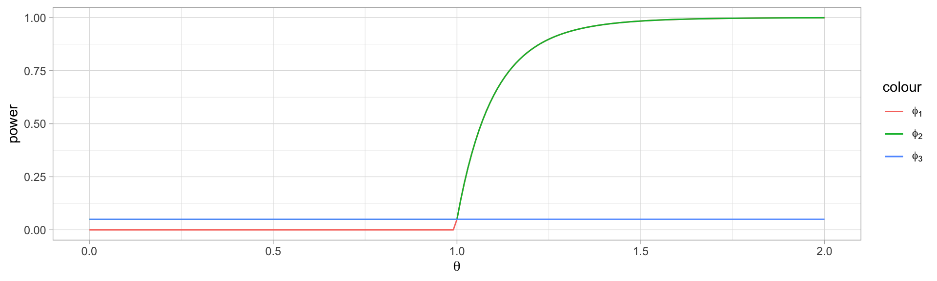
Indeed, the three tests have power functions given by (using \(\alpha=0.05\) and \(n=10\)):
Suppose \(X_1,\dots,X_n\sim Uniform(0,\theta)\) iid. We already established that the pair of order statistics \(X_{(1)}, X_{(n)}\) is minimal sufficient for the corresponding estimation problem, and that the joint density is non-zero (and constant \(1/\theta^n\)) only if \(0\leq X_{(1)}\leq X_{(n)}\leq \theta\).
\(\phi_1\) and \(\phi_2\) are both UMP - since they agree completely in power on all of \(H_a\). However, \(\phi_1\) has better discriminatory ability - it will not reject at all for most of \(H_0\), whereas \(\phi_2\) has a constant risk \(\alpha\) of rejecting \(H_0\) no matter what the true value is.
\(\phi_3\) is the worst of both worlds - it comes nowhere near most powerful on \(H_a\), but it also comes nowhere near a low rejection probability anywhere on \(H_0\). There is a theorem telling us we can (pretty much) always do better than \(\phi_3\).
Two-tailed tests
Consider \(X_1,\dots,X_n\sim\mathcal{N}(\theta,1)\) and hypotheses \(H_0: \theta=\theta_0\) and \(H_a: \theta\neq\theta_0\).
Normal distributed data like this also has monotone likelihood ratios (do you see why?) using the test statistic \(\overline{X}\).
So we can construct separate UMP tests for \(H_a:\theta>\theta_0\) and \(H_a:\theta<\theta_0\) by using \[
\phi_+ = \begin{cases}
1 & \text{if }\overline{x}>c_+ \\
0 & \text{otherwise}
\end{cases}
\qquad
\phi_- = \begin{cases}
1 & \text{if }\overline{x}<c_- \\
0 & \text{otherwise}
\end{cases}
\]
By inspecting the sampling distribution of \(\overline{x}\) given our assumptions, we can conclude that \(c_+=\theta_0 +CDF_{\mathcal{N}(0,1)}^{-1}(1-\alpha)/\sqrt{n}=\theta_0+z_{\alpha}/\sqrt{n}\) and \(c_-=\theta_0-z_\alpha/\sqrt{n}\) should give the expected significance levels.
However, consider some \(\theta_1>\theta_0\) and \(\theta_2<\theta_0\), and lets compute the power of both of these tests at each of these values: \[
\begin{align*}
\EE_{\theta_1}[\phi_+] &= \PP[\overline{x}>\theta_0+z_\alpha/\sqrt{n} | \theta_1]
&\EE_{\theta_2}[\phi_+] &= \PP[\overline{x}>\theta_0+z_\alpha/\sqrt{n} | \theta_2]\\
&= 1-CDF_{\mathcal{N}(\theta_1,1/n)}(\theta_0+z_\alpha/\sqrt{n}) &
&= 1-CDF_{\mathcal{N}(\theta_2,1/n)}(\theta_0+z_\alpha/\sqrt{n}) \\
\EE_{\theta_1}[\phi_-] &= \PP[\overline{x}<\theta_0-z_\alpha/\sqrt{n} | \theta_1]
&\EE_{\theta_2}[\phi_-] &= \PP[\overline{x}<\theta_0-z_\alpha/\sqrt{n} | \theta_2]\\
&= 1-CDF_{\mathcal{N}(\theta_1,1/n)}(\theta_0-z_\alpha/\sqrt{n}) &
&= 1-CDF_{\mathcal{N}(\theta_2,1/n)}(\theta_0-z_\alpha/\sqrt{n}) \\
\end{align*}
\]
Two-tailed tests
Consider \(X_1,\dots,X_n\sim\mathcal{N}(\theta,1)\) and hypotheses \(H_0: \theta=\theta_0\) and \(H_a: \theta\neq\theta_0\).
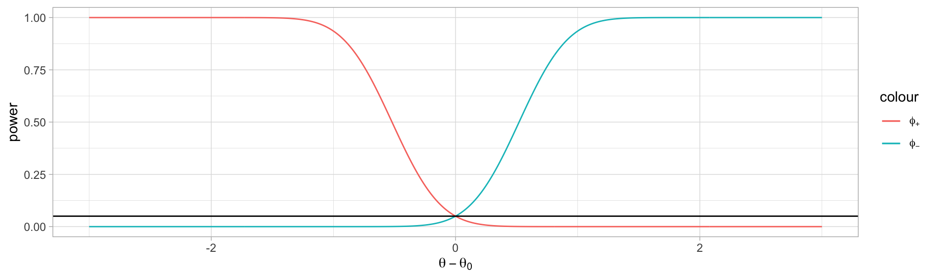
We can view the power functions of both these one-tailed tests:
Notice that the test that we know is UMP for each of the tails is very different from the behavior of the test UMP on the other tail; the methods we have to construct best possible tests break down if we try to do two-tailed testing.
There are ways to construct two-tailed tests when the data comes from an exponential family that are UMP within a family of candidate test functions.
Exponential Family Test Statistics
Theorem
If \(X\) comes from an exponential family with densities
Then the distribution of \(T=T(X)\) has density \(q_\theta(t) = \exp\left[\color{CornflowerBlue}{\boldsymbol{\eta}(\boldsymbol{\theta})}\cdot \color{DarkGreen}{t} - \color{Maroon}{A(\boldsymbol{\theta})}\right]\) times some reference density that does not depend on \(\theta\) or \(t\).
We have a very comfortable criterion to recognize monotone likelihood ratios in exponential families:
Theorem
An exponential family with densities
\[
f(\boldsymbol{x}|\boldsymbol{\theta}) =
\color{DarkGoldenrod}{h(\boldsymbol{x})}\cdot
\exp\left[
\color{CornflowerBlue}{\boldsymbol{\eta}(\boldsymbol{\theta})}\cdot
\color{DarkGreen}{\boldsymbol{T}(\boldsymbol{x})} -
\color{Maroon}{A(\boldsymbol{\theta})}
\right]
\] has monotone likelihood ratios with respect to the test statistic \(T=\color{DarkGreen}{T(x)}\) if \(\color{CornflowerBlue}{\eta(\theta)}\) is an increasing function of \(\theta\).
Proof
Consider \(\theta_1<\theta_2\) and the likelihood ratio
As long as \(\color{CornflowerBlue}{\eta(\theta_2)-\eta(\theta_1)}>0\), this is an increasing function of \(T\), and hence the family has monotone likelihood ratios.
Derive All The Tests
Last week, we saw that \(\overline{X}\) is the key building block for tests for population mean, leading to either normal or T-distributed sampling distributions that we compute thresholds from.
Let’s derive some more test statistics, now that we have tools.
Binomial proportions, known \(n\)
Recall that \(Binomial(n,p)\) is an exponential family, with
\[
f(x|p) = {n\choose x}\exp\left[\log\left(\frac{p}{1-p}\right)\cdot x - n\log(1-p)\right] \\
T(x) = x
\]
Since \(\log(p/(1-p))\) is monotonically increasing, we have monotone likelihood ratios, and so a one-tailed (upper-tailed) UMP is given by \[
\phi(x) = \begin{cases}
1 & \text{if }x > c \\
\gamma & \text{if } x = c \\
0 & \text{if }x < c
\end{cases}
\qquad
\begin{align*}
c &= \max\{x : 1-CDF_{Binomial(n,p)}(x)<\alpha \} \\
\gamma &= \frac{\alpha-(1-CDF(c-1))}{PMF(c)}
\end{align*}
\]
This is exactly the Small-Sample Test described on p. 453 in Section 9.3.
Derive All The Tests
Last week, we saw that \(\overline{X}\) is the key building block for tests for population mean, leading to either normal or T-distributed sampling distributions that we compute thresholds from.
Let’s derive some more test statistics, now that we have tools.
Binomial proportions, known \(n\)
Binomial Proportions, exact small sample test
Null Hypothesis
\(p = p_0\)
Test Statistic
\(X\)
Alternative Hypothesis
Rejection Region for Level \(\alpha\)
Upper Tail
\(X > CDF_{Binomial(n,p_0)}^{-1}(1-\alpha)-1\)
Two-tailed
\(X > CDF_{Binomial(n,p_0)}^{-1}(1-\alpha/2)-1\) or \(X < CDF_{Binomial(n,p_0)}^{-1}(\alpha/2)+1\)
Lower Tail
\(X < CDF_{Binomial(n,p_0)}^{-1}(\alpha)+1\)
Derive All The Tests
Last week, we saw that \(\overline{X}\) is the key building block for tests for population mean, leading to either normal or T-distributed sampling distributions that we compute thresholds from.
Let’s derive some more test statistics, now that we have tools.
Wald Tests
If \(\hat\theta\sim\mathcal{N}(\theta, \sigma_{\hat\theta})\) is any (asymptotically normal) estimator of \(\theta\), we can use it to build a hypothesis test.
This is the Wald construction that gave name to the Wald confidence intervals we saw earlier.
The idea with a Wald test is to generate a large-sample test for upper-, lower- or two-tailed tests of \(H_0:\theta=\theta_0\) by using this normal distribution.
Since \(\hat\theta\sim\mathcal{N}(\theta, \sigma_{\hat\theta})\), it follows that \(\frac{\hat\theta-\theta_0}{\sigma_{\hat\theta}}\sim\mathcal{N}(0,1)\) and that \(\frac{\hat\theta-\theta_0}{s_{\hat\theta}}\overset\approx\sim\mathcal{N}(0,1)\).
So we compare the test statistic \(Z=\frac{\hat\theta-\theta_0}{\sigma_{\hat\theta}}\) or \(T=\frac{\hat\theta-\theta_0}{s_{\hat\theta}}\) to \(z_\alpha\) (or to \(z_{\alpha/2}\) for a two-tailed test).
Derive All The Tests
Last week, we saw that \(\overline{X}\) is the key building block for tests for population mean, leading to either normal or T-distributed sampling distributions that we compute thresholds from.
Let’s derive some more test statistics, now that we have tools.
Large-sample Binomial Test
Let \(X\sim Binomial(n,p)\), large and known \(n\), unknown \(p\).
Since \(\hat{p}\overset\approx\sim\mathcal{N}(p, p(1-p)/n)\) we get a Wald test:
Binomial Proportions, Large-sample approximate test
This approximation requires at least \(np_0\geq 10\) and \(n(1-p_0)\geq 10\).
Exercise 9.63 (hypothesis test for variance)
\(X_1, \dots, X_n\sim\mathcal{N}(0,\sigma^2)\) iid. We are testing \(H_0:\sigma^2=2\) vs. \(H_a:\sigma^2=3\).
Show that a most powerful test rejects \(H_0\) for large values of \(\sum x_i^2\).
This is a case of simple vs. simple testing - both \(H_0\) and \(H_a\) have exactly one random variable. So by the Neyman-Pearson Lemma, the (simple vs simple) likelihood ratio test is UMP.
The test rejects when \(\mathcal{LR}>k\) for some \(k\) chosen to achieve the level \(\alpha\).
Since \(1/4 - 1/6 = (3-2)/12 = 1/12 > 0\), this likelihood ratio increases if \(\sum x_i^2\) increases. So with \(c=\log\left(\left(\frac32\right)^{n/2}k\right)\cdot 12\), the test would reject when \(\sum x_i^2 > c\).
Exercise 9.63 (hypothesis test for variance)
\(X_1, \dots, X_n\sim\mathcal{N}(0,\sigma^2)\) iid. We are testing \(H_0:\sigma^2=2\) vs. \(H_a:\sigma^2=3\).
For \(n=10\), find the value for \(c\) that results in \(\alpha=0.05\).
Our test statistic is \(\sum x_i^2\), and we would need its distribution. Under the null hypothesis, \(x_i \sim \mathcal{N}(0,2)\), so \(x_i/\sqrt{2}\sim\mathcal{N}(0,1)\). It follows that \(\frac{1}{\sqrt{2}}\sum x_i^2\) is a sum of \(n\) independent standard normal variables, so \(\frac{1}{2}\sum x_i^2\sim\chi^2(n)\).
For \(n=10\) and \(\alpha=0.05\), we therefore pick out \(\chi^2_{0.05,10} = CDF^{-1}_{\chi^2(10)}(0.95) \approx 18.3\). Taking the factor \(1/2\) into account, we would reject when \(\sum x_i^2 > 18.3\cdot2\approx 36.6\).
Exercise 9.63 (hypothesis test for variance)
\(X_1, \dots, X_n\sim\mathcal{N}(0,\sigma^2)\) iid. We are testing \(H_0:\sigma^2=2\) vs. \(H_a:\sigma^2=3\).
Is this test UMP for \(H_0:\sigma^2=2\) vs. \(H_a:\sigma^2>2\)?
Yes, since the only fact about \(H_a:\sigma^2=3\) that influenced the derivation was that \(1/2 - 1/3 > 0\), and this would remain true for all \(\sigma^2\in H_a\). The choice of test statistic did not, in the end, depend on the value of \(\sigma^2\) in \(H_a\), and the value of the threshold only depended on \(H_0\).
Exercise 9.64
\(X_1,\dots,X_n\sim\mathcal{D}(\theta)\) with \(PDF_{\mathcal{D}(\theta)}(x) = \theta x^{\theta-1}\), with \(0<x<1\) and \(\theta>0\).
Show that the most powerful test for \(H_0:\theta=1\) vs. \(H_a:\theta=2\) rejects for large values of \(\sum\log x_i\).
We can as an alternative approach observe that \[
\theta x^{\theta-1} = \theta \cdot x^\theta\cdot \frac{1}{x} =
\color{DarkGoldenRod}{\frac{1}{x}}
\cdot\exp\left[
\color{CornflowerBlue}{\theta}\cdot
\color{DarkGreen}{\log x}-
\color{Maroon}{(-\log\theta)}
\right]
\] is an exponential family density. Hence, we know that the joint density replaces \(\color{DarkGreen}{\log x}\) with \(\color{DarkGreen}{\sum\log x_i}\), and that since \(\theta\) is monotonically increasing with \(\theta\), this family has monotonic likelihood ratios, so a likelihood ratio test will reject when \(\color{DarkGreen}{\sum\log x_i}>c\) for some threshold \(c\) chosen to ensure \(\alpha=0.05\).
Is this test UMP for testing \(H_0:\theta=1\) vs. \(H_a:\theta>1\)?
Yes, by the theorems we have explored in this lecture.
If \(n=50\), what would a value of \(c\) be that results in \(\alpha=0.05\)?
At \(n=50\), we are in the realm where we can justify in using Wald tests.
This density function turns out to be a Beta distribution\(Beta(\theta,1)\), and \(-\log x_i\sim Exponential(\theta) = Gamma(1,\theta)\). And since exponential distributions are special cases of Gamma distributions, and Gamma distributions add nicely, we get:
\(-\sum\log x_i\sim Gamma(n,\theta)\), and for \(n=50\) and \(\alpha=0.05\) and \(H_0:\theta=1\), we can use Python or R to compute the threshold value as \(-CDF_{Gamma(50,1)}(0.05)\):