Suppose \(X_1,\dots,X_n\sim\mathcal{N}(\mu,\sigma^2)\), and that \(\sigma^2\) is known.
Suppose further that our null hypothesis is \(\mu=\mu_0\) (a simple hypothesis).
Following Fisher, we might then compute
\[
Z = \frac{\overline{X}-\mu_0}{\sigma/\sqrt{n}}\sim_{H_0}\mathcal{N}(0,1)
\]
If the null hypothesis is true, then\(Z\sim\mathcal{N}(0,1)\). So we can pick a cutoff \(c\) so that \(\PP(Z\geq c) = \alpha\). A typical such \(c\) would be \(z_{\alpha}=1-CDF^{-1}(1-\alpha)\)
Normal Population, Known \(\sigma^2\)
We may ask ourself, for the test with test statistic \(Z=(\overline{X}-\mu_0)/(\sigma/\sqrt{n})\) and with cutoff \(z_\alpha\), what is the power of this test?
For this case, we can with relative ease get a closed formula: \[
\beta(\mu) = \PP(\text{no rejection}|\mu) =
\PP(Z<z_\alpha) = \PP(\overline{X}<\mu_0+z_{\alpha}\sigma/\sqrt{n}) = \\
\PP\left(\frac{\overline{X}-\mu}{\sigma/\sqrt{n}}<\frac{\mu_0-\mu}{\sigma/\sqrt{n}} + \frac{z_\alpha\sigma/\sqrt{n}}{\sigma/\sqrt{n}}\right) =
CDF_{\mathcal{N}(0,1)}\left(z_\alpha+\frac{\mu_0-\mu}{\sigma/\sqrt{n}}\right)
\]
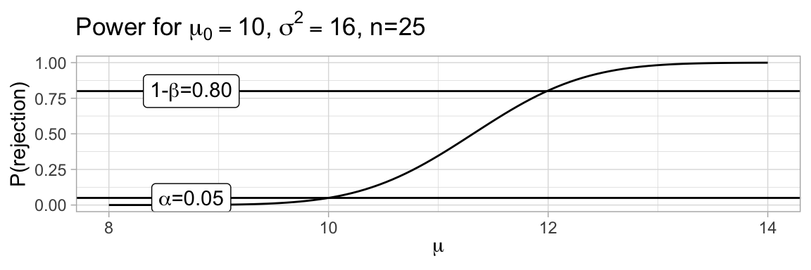
We would get different answers for different hypothetically true distributions (and no answer at all in Fisher’s paradigm), and these can be assembled into a power curve:
With this formula: \(\beta(\mu) = CDF_{\mathcal{N}(0,1)}\left(z_\alpha+\frac{\mu_0-\mu}{\sigma/\sqrt{n}}\right)\), we can compute the sample size needed to get a specified power at a specified degree of separation.
Suppose we wish to be able to detect a true mean of \(\mu=15\) with probability \(80\%\) (ie we need power at 15 to be 0.80), and as in the graph on the last slide, \(\mu_0=10\) and \(\sigma^2=16\). Then, using the threshold from the previous slide, we need:
So for this much smaller distinction, we would need 99 observations for the significance level and statistical power we are looking for.
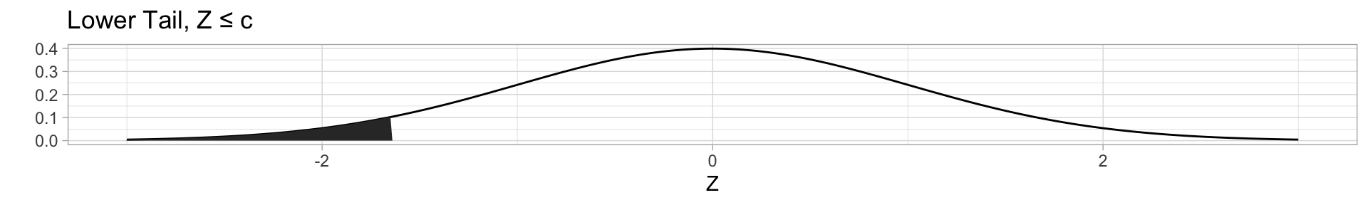
Tailedness
We have three very commonly occurring shapes of rejection regions:
Code
data =tibble(x =seq(-3,3,by=0.01),y =dnorm(x),ylo =ifelse(x<qnorm(0.05), y, 0),yhi =ifelse(x>qnorm(0.95), y, 0),yboth =ifelse(abs(x)>qnorm(0.95), y, 0))ggplot(data, aes(x=x)) +geom_line(aes(y=y)) +geom_area(aes(y=yhi)) +labs(title="Upper Tail, Z ≥ c", x="Z", y="")ggplot(data, aes(x=x)) +geom_line(aes(y=y)) +geom_area(aes(y=yboth)) +labs(title="Two-tailed, |Z| ≥ c", x="Z", y="")ggplot(data, aes(x=x)) +geom_line(aes(y=y)) +geom_area(aes(y=ylo)) +labs(title="Lower Tail, Z ≤ c", x="Z", y="")
Two-tailed threshold values
For two-tailed tests, we distribute the extremal probability mass on two tails of the distribution - so each occurrence of \(z_{\alpha}\) for the one-tailed versions needs to be replaced with a \(z_{\alpha/2}\), since the threshold for the tail needs to contain half the probability mass instead.
Test for \(\mu\), Normal Population, Known \(\sigma^2\)
As long as your null hypothesis is simple, there is a straight-forward way to build a (Fisher-style) test from a pivot:
Given a pivot \(g(\boldsymbol{x}, \theta)\sim\mathcal{D}\) and a single null hypothesis parameter value \(\theta_0\), there is a hypothesis test with test statistic \(G = g(\boldsymbol{x}, \theta_0)\) that rejects with significance level \(\alpha\) if \(\PP_{\mathcal{D}}(\text{observing a value more extreme than }G)\leq\alpha\).
Large Sample Hypothesis Test for the Mean
For large sample sizes (at least \(n>40\)), we can invoke the Central Limit Theorem to claim that \(\overline{X}\overset\approx\sim\mathcal{N}(\mu,\sigma^2/n)\), and invoke the consistency of \(S^2\) as an estimator of \(\sigma^2\) to claim that therefore,
\[
Z =
\frac{\overline{X}-\mu}{S/\sqrt{n}} \overset\approx\sim \mathcal{N}(0,1)
\]
is a pivot. Inserting \(\mu_0\) for \(\mu\), we can derive a hypothesis test from this pivot.
Large Sample Hypothesis Test for the Mean
Large Sample Hypothesis Test for the Mean
Null Hypothesis
\(\mu = \mu_0\)
Test Statistic
\(z = \frac{\overline{x}-\mu_0}{s/\sqrt{n}}\)
Alternative Hypothesis
Rejection Region for Level \(\alpha\)
Upper Tail
\(z>z_{\alpha}\)
Two-tailed
\(|z|>z_{\alpha/2}\)
Lower Tail
\(z<-z_{\alpha}\)
For power calculations and sample sizes, either specify a value for \(\sigma\) and use the formulas for known \(\sigma^2\), or use the methods that we will introduce with the \(T\)-test next.
Duality of Confidence Intervals and Hypothesis Tests
Theorem
Suppose that for every \(\theta_0\in\Theta\) there is a test at level \(\alpha\) of the hypothesis \(H_0: \theta=\theta_0\) with rejection region \(RR(\theta_0)\). Then the set \(C(X) = \{\theta : X\not\in RR(\theta)\}\) is a \(1-\alpha\) confidence set for \(\theta\).
This result inverts, so that from a confidence interval construction \(CI_{1-\alpha}(X)\) we can also create a hypothesis test:
Duality Hypothesis Test
Null Hypothesis
\(H_0: \theta=\theta_0\)
Test Statistic
\(CI_{1-\alpha}(X)\)
Reject \(H_0\) at a significance level \(\alpha\) when
\(\theta_0\not\in CI_{1-\alpha}(X)\)
Small Sample Hypothesis Test for the Mean
Recall that we introduced the T-distribution to deal with the sample distribution of \(\overline{X}\) for small sample sizes. We derived the confidence interval construction:
Note that we get the same result by noticing that \(T=(\overline{X}-\mu)/(S/\sqrt{n})\sim T(n-1)\) is a pivot.
Power Calculation and Sample Sizes for the T-test
Sample distributions for the test statistic \(T\) at a given alternative hypothesis \(\mu\) turn out to be quite difficult computations, best done with numeric integration of the density one might derive for that case.
The book has graphs that can be used to investigate power for these curves.
Alternatively, R has power calculation by standard and Python has power calculation - not in the scipy library, but in the statsmodels library.
R requires you to give values for 4 out of the 5 arguments n, delta (\(\mu_0-\mu\)), power, sd (default 1) and sig.level (default 0.05), and will compute the missing value. To compute required standard deviation, or resulting significance level, you have to explicitly pass in the value NULL for those parameters.