Hypothesis Testing: Background, Error Types

Mikael Vejdemo-Johansson

Hypothesis Testing

\[ \def\RR{{\mathbb{R}}} \def\PP{{\mathbb{P}}} \def\EE{{\mathbb{E}}} \def\VV{{\mathbb{V}}} \]

The Lady Tasting Tea

Ronald Fisher worked at the Rothamstead research farm 1919 - 1933. During his time there, he met Dr. Muriel Bristol and William Roach (who later married each other); offering a cup of tea with milk to Dr. Bristol. She declined, and explained that she preferred the flavor when milk was added before the tea, rather than poured into the tea. Fisher claimed it must surely not make a difference which order tea and milk are poured, and Roach suggested they test it.

Fisher devised a statistical test for the ability to tell the difference between orders, and Roach assisted with cups for Bristol to taste and tell which cups were poured in which order. The event, and the test, are described in Chapter 2 of Fisher’s The Design of Experiments (1935)

In the setup, Fisher poured 4 cups with tea first and 4 cups with milk first, and served the 8 cups in random order. The number of possible sets of 4 cups out of 8 is \({8\choose 4} = 70\), yielding a probability of \(1/70 \approx 0.0143\) of correctly identifying all cups by chance.

16 out of the 70 sets will choose 3 correctly and 1 incorrectly, with a probability of \(17/70 \approx 0.2429\) of choosing at least 3 correctly.

Fisher argues that a probability around 25% is too common to see it as clearly not happening by chance, while a probability around 1.5% is small enough that the reasonable conclusion then must be that Dr. Bristol were able to discern the flavors well enough - in other words, only in the case of Dr. Bristol correctly identifying all cups will he admit that she can taste a difference.

Dr. Bristol tasted all 8 cups and chose 4 for each of the two preparation methods, and correctly identified all 8 cups, proving her capability to taste a difference.

Fisher’s Significance Testing

This example sets (part of) the structure for what developed into modern day hypothesis testing: some statement is formulated representing the claim you are trying to refute. Based on this null hypothesis, you compute some test statistic, and see whether its value falls within a pre-determined rejection region. If it does, you have sufficient evidence to reject the null hypothesis, refuting the claim - and if it does not, you do not.

the null hypothesis is never proved or established, but is possibly disproved, in the course of experimentation. Every experiment may be said to exist only in order to give the facts a chance of disproving the null hypothesis.

the null hypothesis must be exact, that is free from vagueness and ambiguity, because it must supply the basis of the “problem of distribution,”

We may, however, choose any null hypothesis we please, provided it is exact.

The null hypothesis determines the test statistic and our expectations of its sample distribution. And if the observed values of the test statistic are far out in the tails of the distribution, we are justified in rejecting the null.

Notably, Fisher does not discuss alternative hypotheses.

Neyman-Pearson Hypothesis Testing

Jerzy Neyman and Egon Pearson (son to the famous Karl Pearson) followed up on Fisher’s significance testing by developing their own theory of Hypothesis Testing in a series of papers (starting with The Most Efficient Test of Statistical Hypotheses (1933)).

Neyman-Pearson start by considering the case of choosing between two independent hypotheses \(H_0\) and \(H_1\), and use the likelihood ratio \(\mathcal{L}(H_0|\boldsymbol{x}) / \mathcal{L}(H_1 | \boldsymbol{x})\).

Furthermore, with references back to Laplace and a classical question of how many votes in a court of judges should be needed for conviction, Neyman-Pearson draw a distinction between two different sources of error:

1. to reject \(H_0\) when \(H_0\) is in fact true
2. to accept \(H_0\) when \(H_0\) is in fact false

The best test in Neyman-Pearson’s approach would be a procedure that minimizes \(\PP(\text{false acceptance})\) subject to a bound \(\PP(\text{false rejection})<\alpha\) for some \(\alpha\) chosen by the practitioner.

All our faves are problematic

Ronald Fisher (1890 - 1962) was a mathematician, statistician, biologist, geneticist. He worked for 14 years at Rothamsted to analyze crop data collected sinc ethe 1840s, and developed a lot of fundamental statistics, including variance, the ANOVA, significance testing, derived various sampling distributions (for instance the F-distribution).

Fisher was the Galton Professor of Eugenics at University College London, and an editor of the Annals of Eugenics.

When UNESCO in 1952 published an explicitly anti-racist statement on the concept of race, Fisher was invited to comment on it and was one of four scientists (out of 70 commenting) to oppose the statement.

A selection of statisticians

Some names you will keep running into in statistics:

• Francis Galton (1822-1911); cousin to Charles Darwin; correlation, regression toward the mean, questionnaires and survey methods; proponent of scientific racism and eugenics.
• Karl Pearson (1857-1936); biometrics, chi-squared test, standard deviation, correlation, regression, method of moments, p-values, principal component analysis, histograms; also held the Galton Chair of Eugenics and was an editor of the Annals of Eugenics.
• William Gosset / Student (1876-1937); the T-test.
• Ronald Fisher, (1890-1962); variance, ANOVA, significance testing, sampling distributions, p-values, …
• Jerzy Neyman (1894-1981); confidence interval, hypothesis testing
• Egon Pearson (1895-1980); hypothesis testing
• John Tukey (1915-2000); FFT, exploratory data analysis, graphical presentation, jackknife for variance, boxplot
• Calyampudi Radhakrishna Rao (1920-); Rao-Blackwell theorem, Cramér-Rao bound
• Bradley Efron (1938-); bootstrap

Statistical feud

Fisher and Neyman-Pearson clashed hard over their different approaches to testing:

Neyman-Pearson require the explicit choice of the alternatives against which a null hypothesis is tested, which Fisher opposed strongly:

[there is no reason for] believing that a hypothesis has been proved to be true merely because it is not contradicted by the available facts

The frequency of the 1st class [type I error] .. . is calculable and therefore controllable simply from the specification of the null hypothesis. The frequency of the 2nd kind must depend … greatly on how closely they [rival hypotheses] resemble the null hypothesis. Such errors are therefore incalculable . . . merely from the specification of the null hypothesis, and would never have came into consideration in the theory only of tests of significance, had the logic of such tests not been confused with that of acceptance procedures.

As staunch as the opposition (primarily between Neyman and Fisher) was through the years, the distinction has faded and modern day statistical textbooks teach a hybrid of the two approaches.

Hypothesis Testing - definitions

Definition

A hypothesis is a set of random variables. These often come in parametrized families, characterized by sets of admissible parameters.

Definition

A test statistic is some function of sample data used to decide whether or not to reject a null hypothesis \(H_0\).

Definition

A rejection region is the set of all possible values of the test statistic for which \(H_0\) will be rejected.

Definition

A statistical hypothesis test is specified by a test statistic and a rejection region, and refers to the procedure of computing the test statistic and checking whether it falls within the rejection region.

Error Types¹

We distinguish between different types of errors made, and pay attention to the corresponding error probabilities:

		Test outcome
		accept	reject
H0 is…	true	true accept	false reject
	false	false accept	true reject

We define several probabilities, fundamental to studying hypothesis testing:

• The significance level or false positive rate of a test is \(\alpha=\PP(\text{false reject} | H_0\text{ is true})\).
• The false negative rate of a test is \(\beta=\PP(\text{false accept} | H_0\text{ is false})\).
• The power of a test is \(1-\beta = \PP(\text{true accept} | H_0\text{ is false})\)

Note that while \(\alpha\) is usually specified in general, \(\beta\) tends to depend on a choice of a specific alternative to measure power against. This is because null hypotheses are usually either simple or dominated by a simple hypothesis, while alternatives tend to be composite.

1. many use “Type I error” and “Type II error” here, a practice I find confusing and unhelpful

Aside: Confusion Matrix

These quantities are derived from a confusion matrix: given an actual condition that can be Positive or Negative, and a predicted condition that can be Positive or Negative, the (extended) confusion matrix is:

		Predicted condition
	Total population \(P+N\)	Positive (PP)	Negative (PN)	Informedness \(TPR+TNR-1\)	Prevalence threshold (PT) \(\frac{\sqrt{TPR\times FPR}-FPR}{TPR-FPR}\)
Actual condition	Positive (P)	True positive (TP) hit	False negative (FN) type II error, miss, underestimation	True positive rate (TPR) recall, sensitivity, probability of detection, hit rate, power \(\frac{TP}{P}=1-FNR\)	False negative rate (FNR) miss rate \(\frac{FN}{P}=1-TPR\)
	Negative (N)	False positive (FP) type I error, false alarm, overestimation	True negative (TN) correct rejection	False positive rate (FPR) prob. of false alarm, fall-out \(\frac{FP}{N} = 1-TNR\)	True negative rate (TNR) specificity, selectivity \(\frac{TN}{N} = 1-FPR\)
	Prevalence \(\frac{P}{P+N}\)	Positive predictive value (PPV) precision \(\frac{TP}{PP} = 1-FDR\)	False omission rate (FOR) \(\frac{FN}{PN} = 1-NPV\)	Positive likelihood ratio (LR+) \(\frac{TPR}{FPR}\)	Negative likelihood ratio (LR-) \(\frac{FNR}{TNR}\)
	Accuracy (ACC) \(\frac{TP+TN}{P+N}\)	False discovery rate (FDR) \(\frac{FP}{PP}=1-PPV\)	Negative predictive value (NPV) \(\frac{TN}{PN}=1-FOR\)	Markedness (MK) \(PPV + NPV - 1\)	Diagnostic odds ratio (DOR) \(\frac{LR+}{LR-}\)
	Balanced accuracy (BA) \(\frac{TPR+TNR}{2}\)	F1 score \(\frac{2PPV\times TPR}{PPV+TPR} = \frac{2TP}{2TP+FP+FN}\)	Fowlkes-Mallows index (FM) \(\sqrt{PPV\times TPR}\)	Matthews correlation coefficient (MCC) \(\sqrt{TPR\times TNR\times PPV\times NPV}\) \(-\sqrt{FNR\times FPR\times FOR\times FDR}\)	Threat score critical success index, Jaccard index \(\frac{TP}{TP+FN+FP}\)

The Lady Tasting Tea revisited

We can describe The Lady Tasting Tea systematically as follows:

\(H_0\)

All cups are indistinguishable

\(H_a\)

Dr. Bristol can tell the difference¹

Test Statistic \(C\)

Number of cups correctly identified as milk first²

Rejection Region

\(\{4\}\)

Acceptance (Non-rejection) Region

\(\{0,1,2,3\}\)

Significance Level

\(\PP(4 | HyperGeometric(4, 4, 4)) \approx0.0143\)

Power Level

Not considered by Fisher’s Significance Testing

1. Fisher would not have used an alternative hypothesis formulation

2. …or as tea first, pick whichever group you want…

Significance and Power illustrated

Suppose we know our test statistic \(X\sim\mathcal{N}(\mu,\sigma^2)\) for some known \(\sigma^2\), and unknown \(\mu\). Our null hypothesis is specified by \(H_0: \mu = \mu_0\), and our alternative hypothesis is specified as a subset of possible values for \(\mu\) as \(\mu < \mu_0\).

For instance, from Example 9.2, a known type of paint has drying time \(T\sim\mathcal{N}(75, 9^2)\). A new additive is proposed to decrease drying times, and the proposers believe this remains normally distributed with lower mean but retained variance.

We have collected \(T_1,\dots,T_{25}\) from test specimens. We expect \(\overline{T}\sim\mathcal{N}(\mu, 9^2/25\approx3.24)\). A rejection region \(\overline{x}\leq 70.8\) is suggested.

Code

library(tidyverse)
library(latex2exp)
theme_set(theme_light())
x.0 = 70.8

x.true = 75
tibble(x = seq(65, 85, length.out=1001),
       y = dnorm(x, mean=x.true, sd=9/sqrt(25)),
       ylo = ifelse(x<x.0, dnorm(x,mean=x.true,sd=9/sqrt(25)), 0)) %>%
  ggplot(aes(x=x)) +
  geom_line(aes(y=y)) +
  geom_area(aes(y=ylo)) +
  geom_vline(xintercept = x.0) +
  annotate("label", x=70, y=0.05, label=TeX(paste("\\alpha \\approx", round(pnorm(x.0, mean=x.true, sd=9/sqrt(25)), 3)))) +
  scale_x_continuous(breaks=c(65,70,x.0,75,80,85),
                     labels=c(65,"",TeX("T=70.8"),75,80,85))
x.true = 72
tibble(x = seq(65, 85, length.out=1001),
       y = dnorm(x, mean=x.true, sd=9/sqrt(25)),
       ylo = ifelse(x>x.0, dnorm(x,mean=x.true,sd=9/sqrt(25)), 0)) %>%
  ggplot(aes(x=x)) +
  geom_line(aes(y=y)) +
  geom_area(aes(y=ylo)) +
  geom_vline(xintercept = x.0) +
  annotate("label", x=72, y=0.05, label=TeX(paste("\\beta(", x.true,") \\approx", round(1-pnorm(x.0, mean=x.true, sd=9/sqrt(25)), 3)))) +
  scale_x_continuous(breaks=c(65,70,x.0,75,80,85),
                     labels=c(65,"",TeX("T=70.8"),75,80,85))
x.true = 70
tibble(x = seq(65, 85, length.out=1001),
       y = dnorm(x, mean=x.true, sd=9/sqrt(25)),
       ylo = ifelse(x>x.0, dnorm(x,mean=x.true,sd=9/sqrt(25)), 0)) %>%
  ggplot(aes(x=x)) +
  geom_line(aes(y=y)) +
  geom_area(aes(y=ylo)) +
  geom_vline(xintercept = x.0) +
  annotate("label", x=72, y=0.05, label=TeX(paste("\\beta(", x.true,") \\approx", round(1-pnorm(x.0, mean=x.true, sd=9/sqrt(25)), 3)))) +
  scale_x_continuous(breaks=c(65,70,x.0,75,80,85),
                     labels=c(65,"",TeX("T=70.8"),75,80,85))
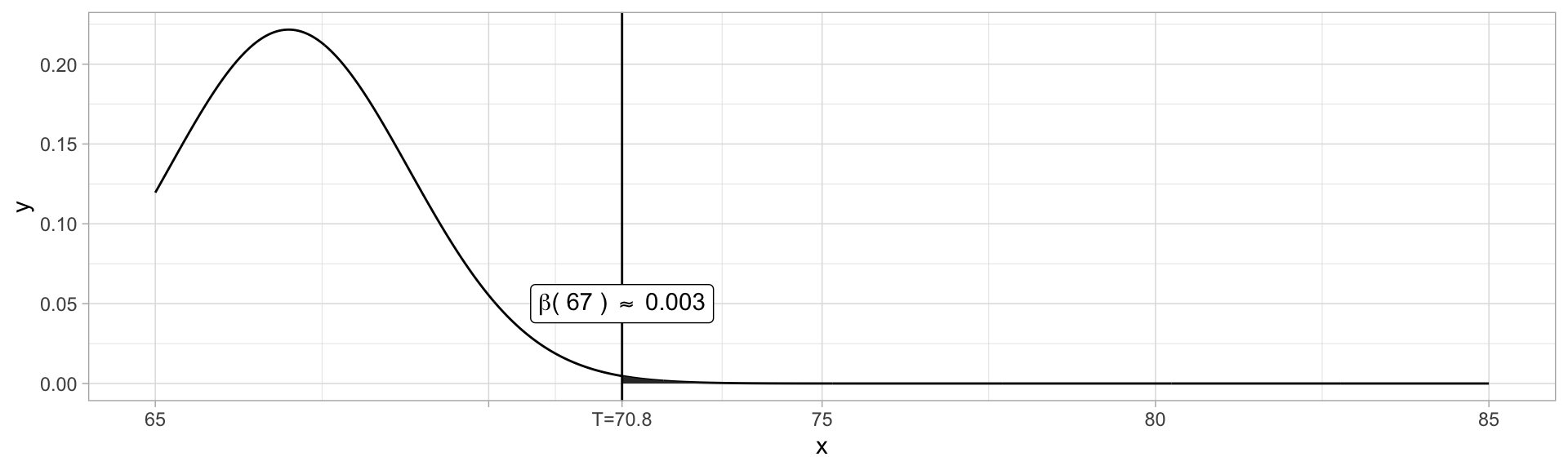
x.true = 67
tibble(x = seq(65, 85, length.out=1001),
       y = dnorm(x, mean=x.true, sd=9/sqrt(25)),
       ylo = ifelse(x>x.0, dnorm(x,mean=x.true,sd=9/sqrt(25)), 0)) %>%
  ggplot(aes(x=x)) +
  geom_line(aes(y=y)) +
  geom_area(aes(y=ylo)) +
  geom_vline(xintercept = x.0) +
  annotate("label", x=72, y=0.05, label=TeX(paste("\\beta(", x.true,") \\approx", round(1-pnorm(x.0, mean=x.true, sd=9/sqrt(25)), 3)))) +
  scale_x_continuous(breaks=c(65,70,x.0,75,80,85),
                     labels=c(65,"",TeX("T=70.8"),75,80,85))

Significance and Power illustrated

Suppose we know our test statistic \(X\sim\mathcal{N}(\mu,\sigma^2)\) for some known \(\sigma^2\), and unknown \(\mu\). Our null hypothesis is specified by \(H_0: \mu = \mu_0\), and our alternative hypothesis is specified as a subset of possible values for \(\mu\) as \(\mu < \mu_0\).

For instance, from Example 9.2, a known type of paint has drying time \(T\sim\mathcal{N}(75, 9^2)\). A new additive is proposed to decrease drying times, and the proposers believe this remains normally distributed with lower mean but retained variance.

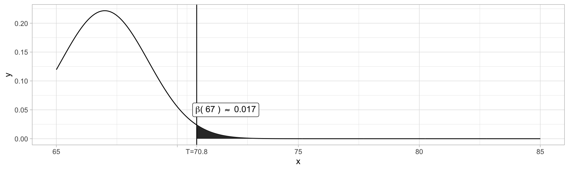
We have collected \(T_1,\dots,T_{25}\) from test specimens. We expect \(\overline{T}\sim\mathcal{N}(\mu, 9^2/25\approx3.24)\). Given the very small \(\alpha\) using \(70.8\), another rejection region \(\overline{x}\leq 72\) is suggested.

Code

library(tidyverse)
library(latex2exp)
theme_set(theme_light())
x.0 = 72

x.true = 75
tibble(x = seq(65, 85, length.out=1001),
       y = dnorm(x, mean=x.true, sd=9/sqrt(25)),
       ylo = ifelse(x<x.0, dnorm(x,mean=x.true,sd=9/sqrt(25)), 0)) %>%
  ggplot(aes(x=x)) +
  geom_line(aes(y=y)) +
  geom_area(aes(y=ylo)) +
  geom_vline(xintercept = x.0) +
  annotate("label", x=70, y=0.05, label=TeX(paste("\\alpha \\approx", round(pnorm(x.0, mean=x.true, sd=9/sqrt(25)), 3)))) +
  scale_x_continuous(breaks=c(65,70,x.0,75,80,85),
                     labels=c(65,"",TeX("T=70.8"),75,80,85))
x.true = 72
tibble(x = seq(65, 85, length.out=1001),
       y = dnorm(x, mean=x.true, sd=9/sqrt(25)),
       ylo = ifelse(x>x.0, dnorm(x,mean=x.true,sd=9/sqrt(25)), 0)) %>%
  ggplot(aes(x=x)) +
  geom_line(aes(y=y)) +
  geom_area(aes(y=ylo)) +
  geom_vline(xintercept = x.0) +
  annotate("label", x=72, y=0.05, label=TeX(paste("\\beta(", x.true,") \\approx", round(1-pnorm(x.0, mean=x.true, sd=9/sqrt(25)), 3)))) +
  scale_x_continuous(breaks=c(65,70,x.0,75,80,85),
                     labels=c(65,"",TeX("T=70.8"),75,80,85))
x.true = 70
tibble(x = seq(65, 85, length.out=1001),
       y = dnorm(x, mean=x.true, sd=9/sqrt(25)),
       ylo = ifelse(x>x.0, dnorm(x,mean=x.true,sd=9/sqrt(25)), 0)) %>%
  ggplot(aes(x=x)) +
  geom_line(aes(y=y)) +
  geom_area(aes(y=ylo)) +
  geom_vline(xintercept = x.0) +
  annotate("label", x=72, y=0.05, label=TeX(paste("\\beta(", x.true,") \\approx", round(1-pnorm(x.0, mean=x.true, sd=9/sqrt(25)), 3)))) +
  scale_x_continuous(breaks=c(65,70,x.0,75,80,85),
                     labels=c(65,"",TeX("T=70.8"),75,80,85))
x.true = 67
tibble(x = seq(65, 85, length.out=1001),
       y = dnorm(x, mean=x.true, sd=9/sqrt(25)),
       ylo = ifelse(x>x.0, dnorm(x,mean=x.true,sd=9/sqrt(25)), 0)) %>%
  ggplot(aes(x=x)) +
  geom_line(aes(y=y)) +
  geom_area(aes(y=ylo)) +
  geom_vline(xintercept = x.0) +
  annotate("label", x=72, y=0.05, label=TeX(paste("\\beta(", x.true,") \\approx", round(1-pnorm(x.0, mean=x.true, sd=9/sqrt(25)), 3)))) +
  scale_x_continuous(breaks=c(65,70,x.0,75,80,85),
                     labels=c(65,"",TeX("T=70.8"),75,80,85))

Interplay between \(\alpha\) and \(\beta\)

Since the Acceptance Region is the complement of the Rejection Region:

• If RR grows, then AR shrinks
• If RR shrinks, then AR grows

Therefore:

• \(\alpha = \PP(RR | H_0)\) will grow if RR grows
• \(\alpha\) will shrink if RR shrinks
• \(\beta = \PP(AR | \text{not } H_0)\) will grow if AR grows
• \(\beta\) will shrink if AR shrinks

Theorem

For fixed experiment, sample size and test statistic, if the rejection region is reduced in order to produce a lower significance level \(\alpha\), then for any parameter value consistent with \(H_a\), \(\beta\) will increase and power of the test will decrease.

Your Homework

8.8a - James Lopez

\[ \begin{align*} -z_{\alpha_1} &<\frac{\overline{x}-\mu}{\sigma/\sqrt{n}} &&< z_{\alpha_2} \\ -z_{\alpha_1}\frac{\sigma}{\sqrt{n}} &< \overline{x}-\mu &&< z_{\alpha_2}\frac{\sigma}{\sqrt{n}} \\ -z_{\alpha_1}\frac{\sigma}{\sqrt{n}}-\overline{x} &< -\mu &&< z_{\alpha_2}\frac{\sigma}{\sqrt{n}}-\overline{x} \\ z_{\alpha_1}\frac{\sigma}{\sqrt{n}}+\overline{x} &> \mu &&> -z_{\alpha_2}\frac{\sigma}{\sqrt{n}}+\overline{x} \\ \end{align*} \]

\(100(1-\alpha)\%\) CI is \(\left(\overline{x}-z_{\alpha_2}\frac{\sigma}{\sqrt{n}},\overline{x}+z_{\alpha_1}\frac{\sigma}{\sqrt{n}}\right)\)

8.8b - James Lopez

\(\alpha = 0.05\),

\[ \begin{align*} \alpha_1 &= \alpha/4 & \alpha_2 &= 3\alpha/4 \\ &= 0.05/4 &&= 3\cdot 0.05/4 \\ &= 0.0125 &&= 0.0375 \end{align*} \]

By using the Z-table, \(z_{0.0125} = 2.24\) and \(z_{0.0375} = 1.78\).

MVJ: or qnorm(1-c(0.0125, 0.0375)) in R or scipy.stats.norm.isf([0.0125, 0.0375]) in Python

In Equation 8.5, \(\alpha_1=\alpha_2=\alpha/2\).

\(-z_{\alpha_1}\frac{\sigma}{\sqrt{n}}+\overline{x}<\mu<z_{\alpha_1}\frac{\sigma}{\sqrt{n}}\color{Maroon}{+\overline{x}}\)

The length is \[ \begin{align*} \left|-z_{\alpha_1}\frac{\sigma}{\sqrt{n}}\right|+\left|z_{\alpha_1}\frac{\sigma}{\sqrt{n}}\right| &=\left|-z_{\alpha/2}\frac{\sigma}{\sqrt{n}}\right|+\left|z_{\alpha/2}\frac{\sigma}{\sqrt{n}}\right| \\ &\approx 1.96\frac{\sigma}{\sqrt{n}} + 1.96\frac{\sigma}{\sqrt{n}} \approx 3.92\frac{\sigma}{\sqrt{n}} \end{align*} \]

In this problem, \(z_{\alpha_1} = z_{0.0125} \approx 2.24\), \(z_{\alpha_2} = z_{0.0375} \approx 1.78\)

\[ \begin{align*} \left|-z_{\alpha_1}\frac{\sigma}{\sqrt{n}}\right|+\left|z_{\alpha_1}\frac{\sigma}{\sqrt{n}}\right| &\approx \left|-2.24\frac{\sigma}{\sqrt{n}}\right| + \left|1.78\frac{\sigma}{\sqrt{n}}\right| \\ &\approx 2.24\frac{\sigma}{\sqrt{n}} + 1.78 \frac{\sigma}{\sqrt{n}} \\ &\approx 4.02\frac{\sigma}{\sqrt{n}} \end{align*} \]

\(4.02\frac{\sigma}{\sqrt{n}} > 3.92\frac{\sigma}{\sqrt{n}}\), so it is wider.

8.10a - Maxim Kleyer

Sample size \(n=15\). Assume mean is \(1/\lambda\)

95% confidence interval: \[ \frac{\chi^2_{1-\alpha/2, 2n}}{2\sum x_i} < \lambda < \frac{\chi^2_{\alpha/2, 2n}}{2\sum x_i} \]

\(\chi^2_{0.975, 30} \approx 16.791\) and \(\chi^2_{0.025,30} \approx 46.979\), \(\sum x_i = 63.2\)

\[ \begin{align*} \frac{16.791}{126.4} &< \lambda < \frac{46.979}{126.4} \\ \\ \frac{126.4}{46.979} &< \frac{1}{\lambda} < \frac{126.4}{16.791} \\ \\ \Rightarrow 2.69 &< \frac{1}{\lambda} < 7.52 \end{align*} \]

8.10b - Maxim Kleyer

99% confidence interval:

\[ \frac{\chi^2_{1-\alpha/2,2n}}{2\sum x_i} < \lambda < \frac{\chi^2_{\alpha/2,2n}}{2\sum x_i} \]

\(\chi^2_{.995,30} \approx 13.787\) and \(\chi^2_{.005,30}\approx 53.672\), \(\sum x_i=63.2\)

\[ \begin{align*} \frac{13.787}{126.4} &< \lambda < \frac{53.672}{126.4} \\ \frac{126.4}{53.672} &< \frac{1}{\lambda} < \frac{126.4}{13.787} \\ \Rightarrow 2.36 &< \frac{1}{\lambda} < 9.168 \end{align*} \]

8.10c - Maxim Kleyer

95% confidence interval for mean is equal to the 95% confidence interval for standard deviation.

So 95% confidence interval for \(\sigma\) is \(2.69 < \sigma < 7.52\).

8.12 - Victoria Paukova

Random sample \(n=110\), \(\overline{x}=.81\), \(S=.34\)

The large sample confidence interval for \(\mu\) is \(\overline{x}\pm z_{\alpha/2}\frac{s}{\sqrt{n}}\)

To calculate a 99% CI for the true \(\mu\), take \(\alpha = 0.01\), \(\alpha/2=0.005\); \(z_{.005} \approx 2.576\)

\[ .81 \pm 2.576\frac{.34}{\sqrt{110}} \approx .7265, .8935 \\ .7265 < \mu < .8935 \]

We are 99% confident that our true mean is between \(.7265\) and \(.8938\), this can be considered an interval width on the slightly wider range.

MVJ: Compare with the result of using the T-distribution with 109 degrees of freedom; where \(t_{.005,109}\approx2.622\):

\[ \overline{x}\pm t_{\alpha/2,n-1}\frac{s}{\sqrt{n}} \\ 0.725 < \mu < 0.895 \]

8.20 - Justin Ramirez

If \(n=4722\), \(p=0.15\) and the confidence level is \(0.99\)

\[ \begin{align*} CI &= \hat{p}\pm E \\ E &= z_{.99}\cdot\sqrt{\frac{p(1-p)}{n}} \\ &\approx 2.58 \cdot \sqrt{\frac{0.15\cdot 0.85}{4722}} \\ &\approx 0.0134 \end{align*} \]

Assuming \(\hat p\approx p\) then \(CI = 0.15 \pm 0.134\):

\[ \boxed{CI = (0.1366, 0.1634)} \]

8.26 - Nicholas Basile

\[ \begin{align*} \sum freq. &= 50 \\ \sum freq. \cdot abs. &= 203 \\ \overline{x} &= \frac{203}{50} = 4.06 \\ CI &= \overline{x}\pm z\sqrt{\frac{\overline{x}}{n}} \\ &\approx 4.06 \pm 1.96\sqrt{\frac{4.06}{50}} \\ &\approx 4.06 \pm .56 \end{align*} \]

\((3.5, 4.6)\) is the CI for \(\lambda\)

8.26 - MVJ

MVJ: Missing here is the actual derivation of the CI:

\[ \color{Maroon}{ \PP(-z_{\alpha/2}<Z<z_\alpha/2) = 1-\alpha\\ \begin{align*} -z_{\alpha/2} < \frac{\overline{x}-\lambda}{\sqrt{\lambda/n}} < z_{\alpha/2} \\ (\overline{x}-\lambda)^2 &< z_{\alpha/2}^2\lambda/n \\ \lambda^2 + (-2\overline{x}-z_{\alpha/2}^2/n)\lambda + \overline{x}^2 &< 0 \\ \lambda &\in \frac{2\overline{x}+z_{\alpha/2}/n\pm\sqrt{(2\overline{x}+z_{\alpha/2}/n)^2-4\overline{x}^2}}{2} \\ &= \overline{x} + z_{\alpha/2}/(2n) \pm \frac{\sqrt{4\overline{x}^2+4\overline{x}z_{\alpha/2}/n+z_{\alpha/2}^2/n^2 - 4\overline{x}^2}}{2} \\ &= \overline{x} + z_{\alpha/2}/(2n) \pm \sqrt{\overline{x}z_{\alpha/2}/n+z_{\alpha/2}^2/(2n)^2} \end{align*} } \]

Which here would yield: \[ 4.06 + 1.96/100 \pm\sqrt{4.06\cdot 1.96/50 + 1.96^2/100^2} \\ \approx (3.6802, 4.479) \]

Alternatively, with the simplifying assumption that \(\overline{x}\approx\lambda\) holds well enough (for one of the \(\lambda\), but not the other one), we get the estimate from the previous slide.