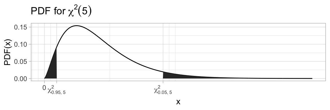
We will write \(\chi^2_{\alpha,\nu}\) for the chi-squared critical value, defining it by \(\chi^2_{\alpha,\nu}=CDF^{-1}_{\chi^2(\nu)}(1-\alpha)\). Since \(\chi^2\) is not a symmetric distribution, there is no short-cut formula to move between low and high quantiles.
Code
library(latex2exp)df =tibble(x=seq(0,25,length.out=1000),y=dchisq(x, 5),ylo=ifelse(pchisq(x,5)<0.05, y, 0),yhi=ifelse(pchisq(x,5)>0.95, y, 0))ggplot(df, aes(x=x)) +geom_line(aes(y=y)) +geom_area(aes(y=ylo)) +geom_area(aes(y=yhi)) +ylab("PDF(x)") +labs(title=TeX("PDF for $\\chi^2(5)$")) +scale_x_continuous(breaks=c(0,qchisq(0.05,5),qchisq(0.95,5)),labels=c("0",TeX("$\\chi^2_{0.95,5}$"),TeX("$\\chi^2_{0.05,5}$")))
A confidence interval for variance
Notice that since \(\frac{(n-1)S^2}{\sigma^2}\sim\chi^2(n-1)\) and \(\chi^2(n-1)\) is not dependent on \(\sigma^2\), this ratio is a pivot for the parameter \(\sigma^2\):
Like before, the assumption of normality of the data is critical to the derivation - much more so here than for the T-distribution. Always check your data with a probability plot / QQ-plot before relying on the confidence interval.
The Bootstrap and Confidence Intervals for everything
We already introduced the bootstrap earlier, as a method for measuring standard error of estimators. The book’s description of the bootstrap in Chapter 7.1 focused on using the estimated parameter for a known parametrized distribution and sampling from that.
Possibly more powerful is the use of the bootstrap without contact with a known distribution form, but just using the data set itself as a proxy for the underlying distribution.
Inherent in the bootstrap as a method is to replace heavy theory with heavy computation, and as such it has taken a while for the bootstrap to come into prominence, but it is a powerful technique that we can use to create sample distributions and confidence intervals by using empirical distributions.
Definition
Given values \(x_1,\dots,x_n\in\mathbb{R}\), the Empirical Cumulative Distribution Function (ECDF) is defined by
Sampling random values from the distribution defined by the ECDF of \(x_1,\dots,x_n\), assuming that the \(x_i\) were iid sampled from a larger (unknown) population, yields the same distribution of samples as sampling from \(\{x_1,\dots,x_n\}\) with replacement.
Example - Billionaires in South Sweden
The Swedish newspaper Expressen published in August 2019 a list of individuals with connections to South Sweden with an income of over 1 billion SEK (ie over about 100M$).
name
age
worth
Mats Paulsson
74
1.0
Anita Paulsson
56
1.2
Zlatan Ibrahimovic
37
1.3
Henrik Persson Ekdahl
38
1.3
Sven Philip-Sörensen
76
1.3
Bengt Hjelm
75
1.5
Pär Sandå
53
1.5
Benny Andersson
71
1.6
Leif Gustavsson
73
1.7
Bo Larsson
73
1.7
Per Sandberg
56
2.0
Gösta Welandsson
81
2.2
Nils-Olov Jönsson
84
2.3
Lisbeth Rausing
58
2.4
Inge Thulin
64
2.5
Gerteric Lindquist
NA
2.5
Sigrid Rausin
56
2.7
Hans-Kristian Rausing
55
2.7
Martin Gren
56
2.7
Gerard de Geer
71
2.9
name
age
worth
Erik Penser
76
2.9
Laurent Leksell
65
3.0
Bicky Chakraborty
75
3.0
Sante Dahl
64
3.0
Lars-Magnus Claesson
69
3.0
Johan Claesson
67
3.0
Christer Brandberg
76
4.0
Dan Olofsson
68
4.0
Jenny Lindén Urnes
47
4.0
Sten Mörtstedt
78
4.0
Eva Lundin
84
6.0
Mona Hamilton
56
6.0
Lukas Lundin
60
6.0
Fredrik Paulsson
46
7.0
Ian Lundin
58
9.0
Rune Andersson
74
9.0
Rutger Arnhult
51
10.0
Peter Kamprad
54
10.0
Jonas Kamprad
52
10.0
Mathias Kamprad
49
10.0
name
age
worth
Erik Paulsson
77
13
Thomas Sandell
57
14
Carl Bennet
67
25
Ane Uggla
70
39
Bertil Hult
77
41
Kirsten Rausing
66
52
Finn Rausing
63
52
Jörn Rausing
58
56
Antonia Ax:son Johnson
75
58
Fredrik Paulsen
66
66
Melker Schörling
71
68
Hans Rausing
92
110
Example - Billionaires in South Sweden
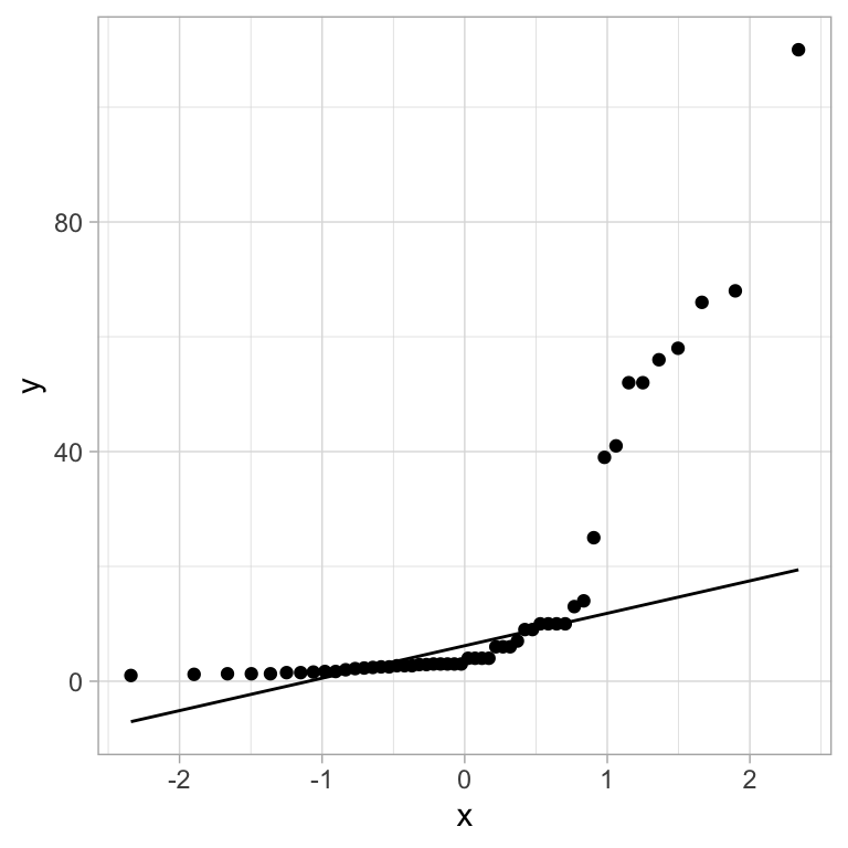
Looking at the income distribution with a QQ-plot, it is clearly not normal:
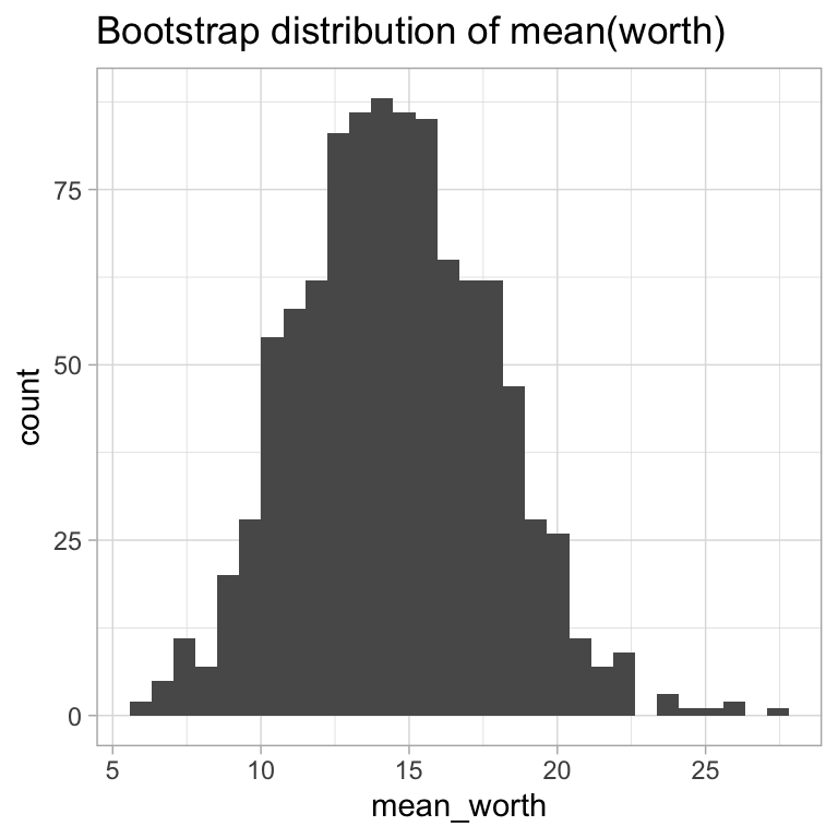
Since it is not normally distributed, and since the departure is pretty dramatic in the upper tail, our methods for confidence intervals are unlikely to work well here. But we can probably get a good result with something that is not as distribution dependent - such as the bootstrap.
Code
library(foreach)sydsvenska.bs.mean =foreach(i=1:1000, .combine=rbind) %do% (sydsvenska %>%slice_sample(prop=1.0, replace=TRUE) %>%summarise(mean_worth =mean(worth)))ggplot(sydsvenska.bs.mean) +geom_histogram(aes(x=mean_worth)) +labs(title="Bootstrap distribution of mean(worth)")
Example - Billionaires in South Sweden
Looking at the income distribution with a QQ-plot, it is clearly not normal:
There is also an argument to be made that maybe the mean is not the most appropriate invariant for a distribution (like personal incomes) that is likely to have very large outliers.
And we have not developed any confidence intervals for the median yet.
But the bootstrap doesn’t care - it can take whatever1 statistic we need to use.
Once we have our bootstrap sample, there are several ways that can be used for creating confidence intervals:
Normal Bootstrap: As long as we have reason to believe that the sample distribution is normal, we can use \(\hat\theta\pm z_{\alpha/2} \hat s_{\hat\theta}\), where \(\hat s_{\hat\theta}\) is the standard error estimated as the standard deviation of the bootstrap distribution.
Basic bootstrap: We can use \(\hat\theta-\theta\) as a pivot, with the bootstrap distribution as the known independent distribution. This gives us the interval \((\hat\theta-(\hat\theta^*_{1-\alpha/2}-\hat\theta), \hat\theta-(\hat\theta^*_{\alpha/2}-\hat\theta)) = (2\hat\theta-\hat\theta^*_{1-\alpha/2}, 2\hat\theta-\hat\theta^*_{\alpha/2})\).
Percentile bootstrap: We can use the percentiles of the bootstrap distribution directly for our confidence interval. This gives us the interval \((\hat\theta^*_{\alpha/2}, \hat\theta^*_{1-\alpha/2})\).
Studentized bootstrap: With our samples we can compute the Student T-statistic for each sample, and use the results as an empirical T-distribution and compute T-distribution thresholds from that. From the bootstrap sample statistics \(\hat\theta^*\) compute \(\hat s_{\hat\theta}\) as for the normal bootstrap. Then compute the bootstrap t-statistics \(t^*=(\hat\theta^*-\hat\theta)/\hat{s}_{\hat\theta}\). From the sample distribution of the bootstrap t-statistics, estimate the quantiles \(t^*_{\alpha/2}\) and \(t^*_{1-\alpha/2}\) to produce the studentized bootstrap confidence interval \((\hat\theta-t^*_{1-\alpha/2}\hat{s}_{\hat\theta}, \hat\theta-t^*_{\alpha/2}\hat{s}_{\hat\theta})\).
Here, we write \(\hat\theta^*_\alpha\) for the \(\alpha\) quantile of the bootstrap distribution, and use \(z_\alpha\) as before.
Example - Billionaires in South Sweden
Inspecting the mean and median bootstrap distributions, we can see that the mean is near normal (with some slight departures), and the median is far from normal.
Code
ggplot(sydsvenska.bs.mean.median,aes(sample=value)) +geom_qq() +geom_qq_line() +facet_wrap(~name, scales="free") +labs(title="Bootstrap distributions normal QQ")
Normal Bootstrap:
Basic Bootstrap:
Percentile Bootstrap:
Studentized Bootstrap:
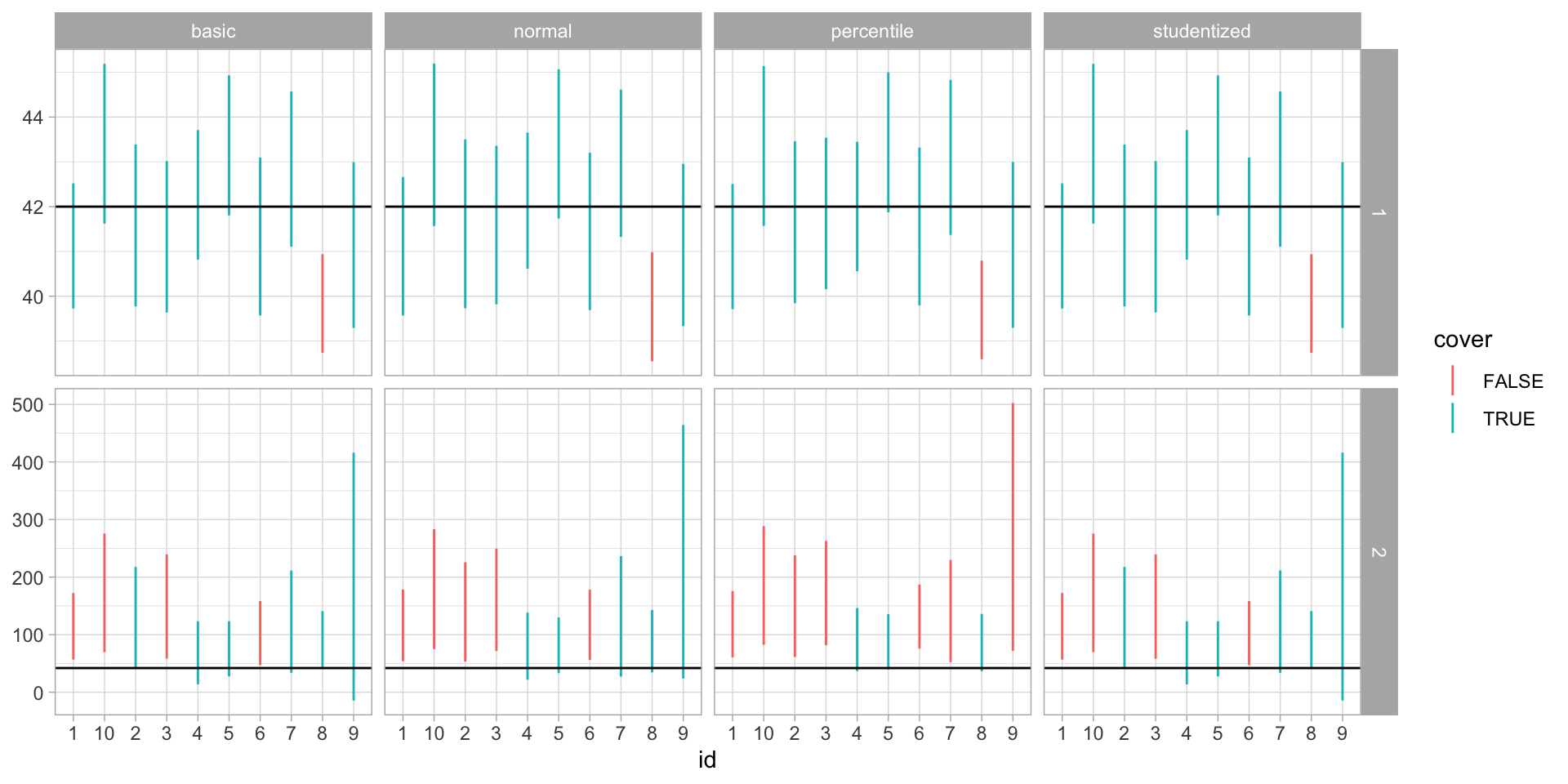
Coverage of the different bootstrap approaches.
Case 1: \(X_1,\dots,X_{30}\sim\mathcal{N}(42,5^2)\).
Case 2: \(X_1,\dots,X_{30}\sim LogNormal(42,5^2)\).
We repeat draws from each distribution 100 times, and for each draw compute bootstrap intervals with all four methods.
Scott: Data Science in R: A Gentle Introduction states:
You can safely bootstrap most common summary statistics most of the time, assuming your observations can plausibly be interpreted as independent samples from some larger reference population. […] These “safe” statistics include […] :
means and medians
standard deviations and inter-quartile ranges
correlations
quantiles of a distribution that aren’t too extreme (e.g. the 25th percentile is OK, but the 99th percentile might not work well unless your sample size is huge)
regression coefficients from ordinary least squares (i.e. from lm in R)
group-wise differences of any of these statistics
[…] Some other examples of where the bootstrap breaks […] include the following situations:
your sample is very small, say less than 20 or maybe 30.
you want to estimate the extreme quantiles of a distribution (of which the min and max are the most extreme possible, as you’ve seen).
your data points are highly correlated across space or time.
you’re fitting a very fancy machine-learning model, with a cool name like “lasso” or “deep neural network.”
the underlying population distribution is very heavy-tailed.
Exercise 8.70 a. - Revisiting \(Uniform(0,\theta)\)
\(X_1,\dots,X_n\sim Uniform(0,\theta)\). We have established an MLE is given by \(X_{(n)}=\max X_i\). Write \(U=X_{(n)}/\theta\). The density of \(U\) is \[
PDF_U(u) =
\begin{cases}
nu^{n-1} & 0\leq u\leq 1 \\
0 & \text{otherwise}
\end{cases}
\] a. \[
\begin{align*}
\PP\left(
(\alpha/2)^{1/n}\leq U \leq (1-\alpha/2)^{1/n}
\right) &=
\int_{(\alpha/2)^{1/n}}^{(1-\alpha/2)^{1/n}}PDF(u)du \\
&= \int_{(\alpha/2)^{1/n}}^{(1-\alpha/2)^{1/n}} nu^{n-1}du \\
&= \left[u^n\right]_{(\alpha/2)^{1/n}}^{(1-\alpha/2)^{1/n}} = \\
&= (1-\alpha/2) - (\alpha/2) = 1 - 2\alpha/2 = 1-\alpha
\end{align*}
\]
We get a CI by using these bounds in simultaneous inequalities: \[
\begin{align*}
(\alpha/2)^{1/n} &\leq U &
U &\leq (1-\alpha/2)^{1/n} \\
(\alpha/2)^{1/n} &\leq X_{(n)}/\theta &
X_{(n)}/\theta &\leq (1-\alpha/2)^{1/n} \\
\theta &\leq X_{(n)}/(\alpha/2)^{1/n} &
X_{(n)}/(1-\alpha/2)^{1/n} &\leq \theta
\end{align*}
\]
So a \(1-\alpha\) CI is given by \[
\left(
\frac{X_{(n)}}{(1-\alpha/2)^{1/n}},
\frac{X_{(n)}}{(\alpha/2)^{1/n}},
\right)
\]
Exercise 8.70 b. - Revisiting \(Uniform(0,\theta)\)
\(X_1,\dots,X_n\sim Uniform(0,\theta)\). We have established an MLE is given by \(X_{(n)}=\max X_i\). Write \(U=X_{(n)}/\theta\). The density of \(U\) is \[
PDF_U(u) =
\begin{cases}
nu^{n-1} & 0\leq u\leq 1 \\
0 & \text{otherwise}
\end{cases}
\]
\[
\begin{align*}
\PP\left(
\alpha^{1/n} \leq U \leq 1
\right) &=
\int_{\alpha^{1/n}}^1 PDF(u) du \\
&= \int_{\alpha^{1/n}}^1 nu^{n-1} du \\
&= \left[u^n\right]_{\alpha^{1/n}}^1 nu^{n-1} = 1 - \alpha
\end{align*}
\]
We can derive a \(1-\alpha\) CI from simultaneous inequalities \[
\begin{align*}
\alpha^{1/n} &\leq U &
U & \leq 1 \\
\alpha^{1/n} &\leq X_{(n)}/\theta &
X_{(n)}/\theta & \leq 1 \\
\theta &\leq X_{(n)}/\alpha^{1/n} &
X_{(n)} \leq \theta
\end{align*}
\]
So a \(1-\alpha\) CI is given by \[
\left(
X_{(n)},
\frac{X_{(n)}}{\alpha^{1/n}}
\right)
\]
Exercise 8.70 c. - Revisiting \(Uniform(0,\theta)\)
\(X_1,\dots,X_n\sim Uniform(0,\theta)\). We have established an MLE is given by \(X_{(n)}=\max X_i\). Write \(U=X_{(n)}/\theta\).
We have derived two confidence intervals: \[
\left(
\frac{X_{(n)}}{(1-\alpha/2)^{1/n}},
\frac{X_{(n)}}{(\alpha/2)^{1/n}},
\right)
\qquad
\left(
X_{(n)},
\frac{X_{(n)}}{\alpha^{1/n}}
\right)
\]
For the data \(x=[4.2, 3.5, 1.7, 1.2, 2.4]\) given in the exercise, we can compute \(n=5\), \(X_{(5)}=4.2\), producing CIs:
We introduce the non-central t distribution, parametrized by degrees of freedom and an offset \(\delta\).
Theorem
If \(Z\sim\mathcal{N}(0,1)\) and \(X\sim\chi^2(\nu)\), then \[
T=\frac{Z+\mu}{\sqrt{X/\nu}}
\sim T_{nc}(\nu, \mu)
\] follows the non-central T-distribution with \(\nu\) degrees of freedom and noncentrality parameter \(\mu\).
This distribution is available in R as dt(x,df,ncp), pt(x,df,ncp) and qt(p,df,ncp) (for abs(ncp)≤37.62) with no random value generators and in Python as scipy.stats.nct.
Theorem
The quantity \[
T=
\frac
{\frac{\overline{X}-\mu}{\sigma/\sqrt{n}}-z_q\sqrt{n}}
{S/\sigma} \sim
T_{nc}(n-1, -z_q\sqrt{n})
\] where \(z_q = CDF_{\mathcal{N}(0,1)}^{-1}(q)\) is the \(q\)th quantile of the standard normal distribution.
We can use this as a pivot for the quantile with critical values \(t_{\alpha/2,\nu,\delta}\) and \(t_{1-\alpha/2,\nu,\delta}\). The \(q\)th quantile of \(\mathcal{N}(\mu,\sigma^2)\) is given by \(x_q = \mu + \sigma z_q\). So we can solve from simultaneous inequalities \[
\begin{align*}
t_{\alpha/2,n-1,-z_q\sqrt{n}} &\leq
\frac{\overline{X}-x_q}{S/\sqrt{n}} &
\frac{\overline{X}-x_q}{S/\sqrt{n}} &\leq
t_{1-\alpha/2,n-1,-z_q\sqrt{n}} \\
\overline{X}-t_{\alpha/2,n-1,-z_q\sqrt{n}}S/\sqrt{n} &\geq x_q &
x_q &\geq \overline{X}-t_{1-\alpha/2,n-1,-z_q\sqrt{n}}S/\sqrt{n}
\end{align*}
\]
So for the \(q\)th quantile of a normal distributed variable, we get the confidence interval \[
x_q\in\left(
\overline{X}-t_{1-\alpha/2,n-1,-z_q\sqrt{n}}S/\sqrt{n},
\overline{X}-t_{\alpha/2,n-1,-z_q\sqrt{n}}S/\sqrt{n}
\right)
\]
For the 5th percentile of beer alcohol from the data in Example 8.11, we can compute a 95% confidence interval as follows:
Code
import numpy as npimport scipy as spimport scipy.stats as spsbeer = np.array([4.68,4.13,4.80,4.63,5.08,5.79,6.29,6.79,4.93,4.25,5.70,4.74,5.88,6.77,6.04,4.95])nct = sps.nct(df=len(beer)-1, nc=-np.sqrt(len(beer))*sps.norm.ppf(0.05))[beer.mean() - nct.ppf(0.975)*beer.std()/np.sqrt(len(beer)), beer.mean() - nct.ppf(0.025)*beer.std()/np.sqrt(len(beer))]
[3.088476047431482, 4.484622271835915]
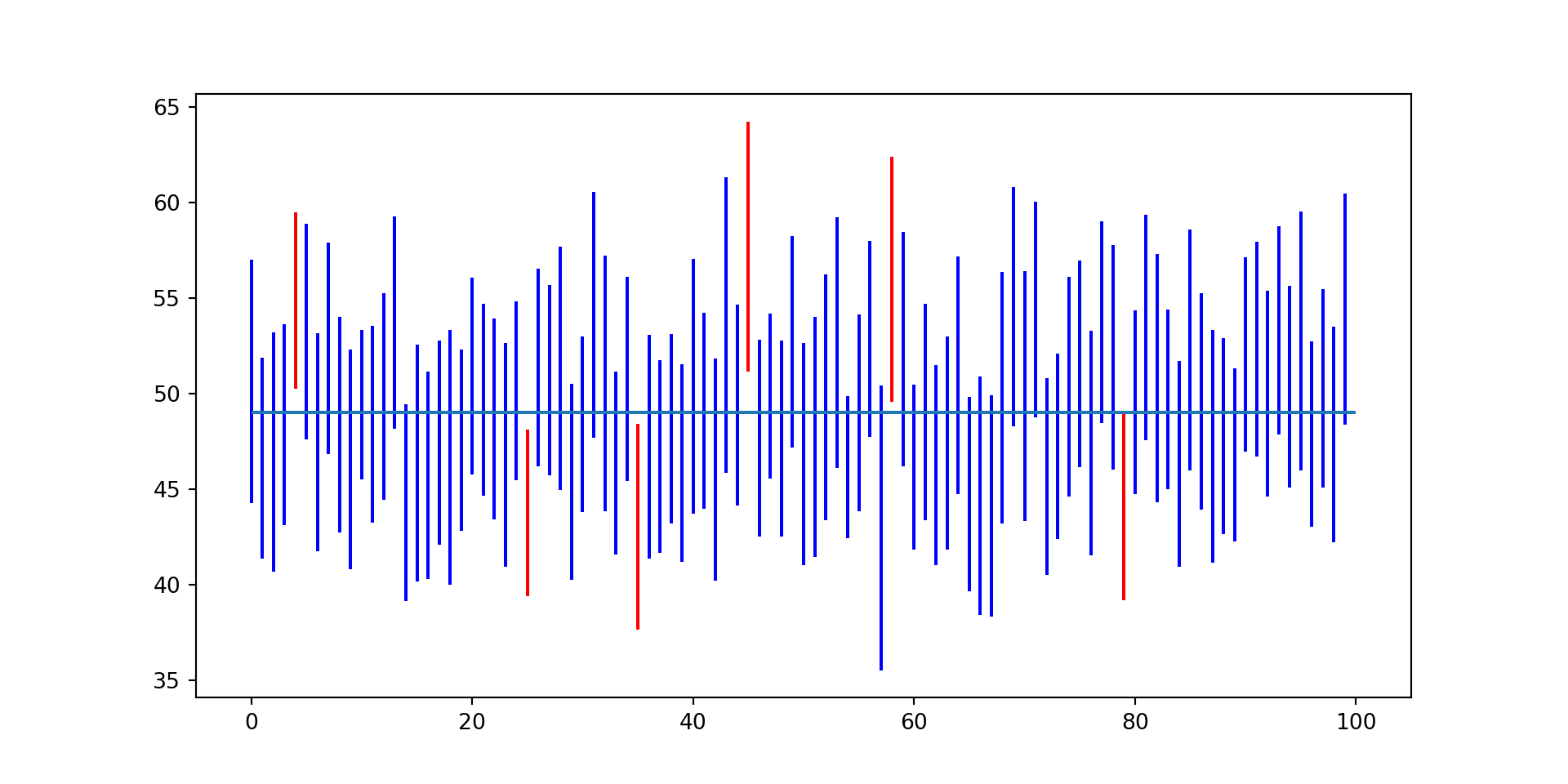
Coverage rates for the quantile confidence intervals
Code
import numpy as npimport scipy as spimport scipy.stats as spsimport matplotlibfrom matplotlib import pyplotimport seabornimport pandasdef qci_lo(x, q, alpha=0.05): nct = sps.nct(df=len(x)-1, nc=-np.sqrt(len(x))*sps.norm.ppf(q))return x.mean() - nct.ppf(1-alpha/2)*x.std()/np.sqrt(len(x))def qci_hi(x, q, alpha=0.05): nct = sps.nct(df=len(x)-1, nc=-np.sqrt(len(x))*sps.norm.ppf(q))return x.mean() - nct.ppf(alpha/2)*x.std()/np.sqrt(len(x))mu =42sigma =17ndist = sps.norm(mu,sigma)z_66 = ndist.ppf(0.66)samples = [ndist.rvs(40) for i inrange(100)]cis = pandas.DataFrame({"lo": [qci_lo(s, 0.66) for s in samples],"hi": [qci_hi(s, 0.66) for s in samples] })cis["cover"] = np.logical_and((cis.lo < z_66), (z_66 < cis.hi))pyplot.vlines(range(len(cis)), cis.lo, cis.hi, [{True: "blue", False: "Red"}[c] for c in cis.cover])pyplot.hlines([z_66],[0],[len(cis)])pyplot.show()