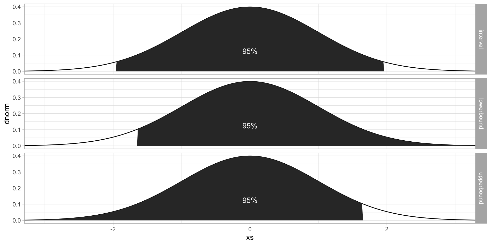
We then talk about upper or lower confidence bounds. These are computed using \(z_\alpha = CDF^{-1}(1-\alpha)\) instead of \(z_{\alpha/2}\), and from a pivot expression involving just one inequality.
Small Samples: Student’s T Distribution
Normal Random Sample Distributions (Ch. 6.4)
Chapter 6.4 introduces several important distributions relating directly to the behavior of normal random samples. Suppose here that \(Z, Z_1,\dots,Z_n\sim\mathcal{N}(0,1)\) iid.
\(Z^2 \sim \chi^2(1)\)
If \(X_1\sim\chi^2(\nu_1)\) and \(X_2\sim\chi^2(\nu_2)\) then \(X_1+X_2\sim\chi^2(\nu_1+\nu_2)\).
So \(Z_1^2+\dots+Z_n^2\sim\chi^2(n)\)
If \(X\sim\mathcal{N}(\mu,\sigma^2)\), then the MLE \(\hat\sigma^2=\frac{1}{n}\sum(X_i-\mu)^2\) is connected to a chi-squared random variable: \((X-\mu)/\sigma \sim \mathcal{N}(0,1)\), and so we get a sum of squares of random variables: \[
\frac{n\hat\sigma^2}{\sigma^2} = \sum\left(\frac{X_i-\mu}{\sigma}\right)^2 \sim\chi^2(n)
\]
Normal Random Sample Distributions (Ch. 6.4)
Chapter 6.4 introduces several important distributions relating directly to the behavior of normal random samples. Suppose here that \(Z, Z_1,\dots,Z_n\sim\mathcal{N}(0,1)\) iid.
\(Z^2 \sim \chi^2(1)\)
If \(X_1\sim\chi^2(\nu_1)\) and \(X_2\sim\chi^2(\nu_2)\) then \(X_1+X_2\sim\chi^2(\nu_1+\nu_2)\).
So \(Z_1^2+\dots+Z_n^2\sim\chi^2(n)\)
It is even true that if \(X_1\sim\chi^2(\nu_1)\) and \(X_3 = X_1+X_2\) with \(X_3\sim\chi^2(\nu_3)\) with \(\nu_r>\nu_1\) and \(X_1,X_2\) independent, then \(X_2\sim\chi^2(\nu_3-\nu_1)\)
We can also consider \[
\sum(X_i-\mu)^2 = \sum[(X_i-\overline{X})+(\overline{X}-\mu)]^2 =\\
= \sum(X_i-\overline{X})^2 + \color{DarkMagenta}{2(\overline{X}-\mu)\sum(X_i-\overline{X})} + \sum(\overline{X}-\mu)^2
\] The middle term vanishes because \(\sum(X_i-\overline{X}) = \sum X_i-n\overline{X} = n\overline{X}-n\overline{X}=0\). Divide through by \(\sigma^2\): \[
\sum\left(\frac{X_i-\mu}{\sigma}\right)^2 =
\sum\left(\frac{X_i-\overline{X}}{\sigma}\right)^2 + n\left(\frac{\overline{X}-\mu}{\sigma}\right)^2 =
\frac{(n-1)S^2}{\sigma^2} + \left(\frac{\overline{X}-\mu}{\sigma/\sqrt{n}}\right)^2
\]
Since \(\overline{X}\sim\mathcal{N}(\mu,\sigma^2/n)\), with \(X_3=\sum\left(\frac{X_i-\mu}{\sigma}\right)^2\sim\chi^2(n)\) and \(X_1=\left(\frac{\overline{X}-\mu}{\sigma/\sqrt{n}}\right)^2\sim\chi^2(1)\) we get that \(X_2=(n-1)S^2/\sigma^2\sim\chi^2(n-1)\).
Normal Random Sample Distributions (Ch. 6.4)
In the previous two slides we have tacitly used a result telling us that \(\overline{X}\) is independent of \(S^2\), which holds for normal distributions but not necessarily non-normal distributions.
Suppose \(Z\sim\mathcal{N}(0,1)\) and \(X\sim\chi^2(\nu)\) are independent random variables. Student’s T-distribution with \(\nu\) degrees of freedom is defined as the distribution of the ratio
\[
T = \frac{Z}{\sqrt{X/\nu}}
\]
It turns out that this distribution has PDF given by (Helmert (1875-1876), Lüroth (1876), Pearson (1895), Student (1908)) \[
PDF(t) = \frac{\Gamma\left(\frac{\nu+1}{2}\right)}{\sqrt{\nu\pi}\Gamma\left(\frac{\nu}{2}\right)}\left(1+\frac{t^2}{\nu}\right)^{-(\nu+1)/2}
\]
The resulting curve looks like a heavy-tailed normal distribution, and can be accessed in R using dt, pt, qt, rt and in Python using scipy.stats.t.
Sidebar: The Student in Student’s T
William Sealy Gosset worked at the Guinness brewery and was studying the barley sources used for beer production. He collaborated with Ronald Fisher to develop a method that could work for potentially very small sample sizes, and published his method.
At the time, the brewery had had relatively recent problems with leaks of industrial secrets through scientific publication and had a blanket ban on publishing for their staff. Gosset convinced the company leadership that these results contain no industrial secrets, but to prevent envy among the other staff engineers, they required him to publish pseudonymously.
So in the journal Biometrika in 1908 appeared the article The Probable Error of a Mean, written by “Student” developing the T-distribution and a corresponding set of statistical tests.
Student’s T and CIs of normal variables
Theorem
If \(X_1,\dots,X_n\sim\mathcal{N}(\mu,\sigma^2)\) iid, then \[
T = \frac{\overline{X}-\mu}{S/\sqrt{n}} \sim T(n-1)
\]
since \(\overline{X}\sim\mathcal{N}(\mu,\sigma^2/n)\), the numerator is a standard normal random variable.
as previously derived, \((n-1)S^2/\sigma^2\sim\chi^2(n-1)\)
So with \(Z=(\overline{X}-\mu)/(\sigma/\sqrt{n})\), \(X=(n-1)S^2/\sigma^2\) and \(\nu=n-1\), we have fully matched the ratio form defining a T-distribution variable.
Confidence Intervals for normal distributions
We have concluded that \(T = (\overline{X}-\mu)/(S/\sqrt{n})\sim T(n-1)\). Notice that even without knowing \(\sigma^2\), this forms a pivot quantity for \(\mu\).
Just like the standard normal, each T-distribution is symmetric around 0, unimodal1. The limit as the DoF\(\to\infty\) is the normal distribution.
Write \(t_{\alpha,\nu}=CDF^{-1}_{T(\nu)}(1-\alpha)\) for the critical value with an upper tail of constant probability mass \(\alpha\).
We get, for \(X_1,\dots,X_n\sim\mathcal{N}(\mu,\sigma^2)\): \[
\PP(-t_{\alpha/2, n-1}<T<t_{\alpha/2,n-1}) = 1-\alpha
\] And thus have to solve the simultaneous inequalities \[
\begin{align*}
-t_{\alpha/2, n-1}&<\frac{\overline{X}-\mu}{S/\sqrt{n}} &
\frac{\overline{X}-\mu}{S/\sqrt{n}} &< t_{\alpha/2,n-1} \\
-t_{\alpha/2, n-1}S/\sqrt{n} &< \overline{X}-\mu &
\overline{X}-\mu &< t_{\alpha/2, n-1}S/\sqrt{n} \\
-(\overline{X}+t_{\alpha/2, n-1}S/\sqrt{n}) &<-\mu &
-\mu &< -(\overline{X}-t_{\alpha/2, n-1}S/\sqrt{n})
\end{align*}
\]
Which gives us the confidence interval \(\mu\in\overline{X}\pm t_{\alpha/2, n-1}S/\sqrt{n}\)
Alert: Our derivation assumes the \(X_i\) are normally distributed. Check your data with eg a QQ-plot (especially for small \(n\)) before applying this CI.
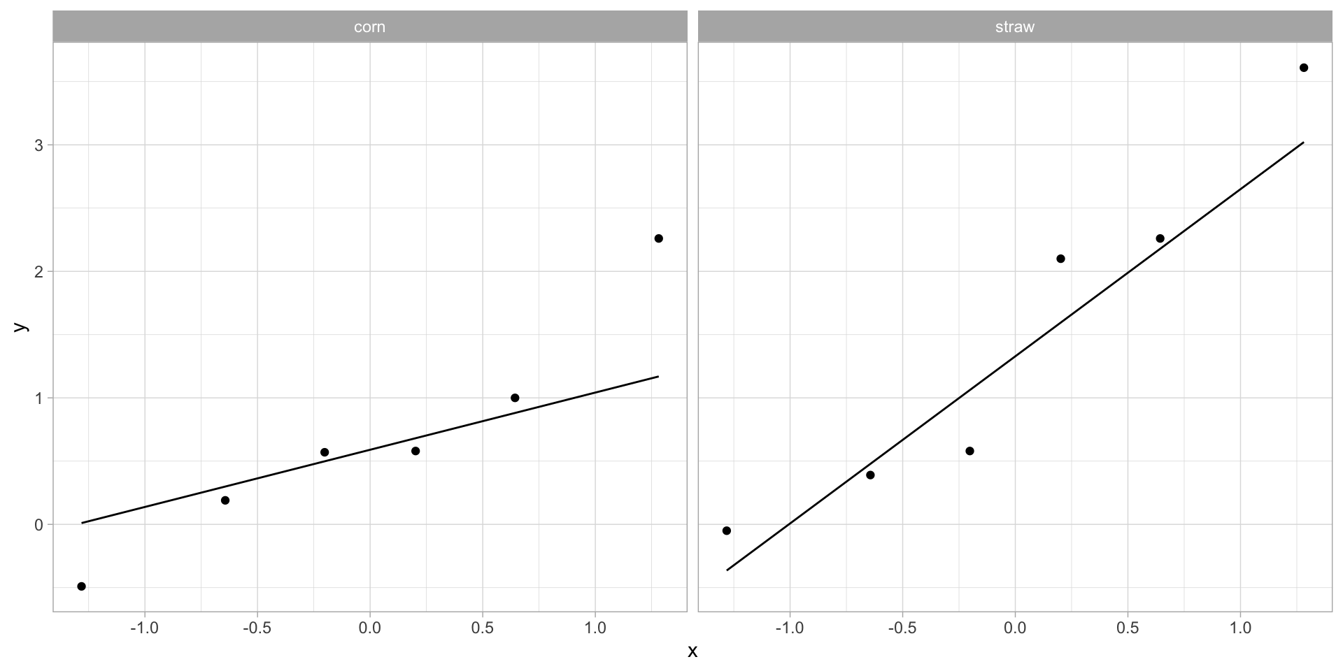
Example (Illustration II from Student (1908))
Sample seed corn from both hard (glutinous) wheat and soft (starchy) wheat were picked in three successive years and planted in heavy and light soil.
Voelcker who ran the initial experiment was looking for whether heavy soil would consistently produce hard corn, and was able to show this, but Student notices that the soft seeds tended to produce high yields. He gives the following data extracted from Voelcker’s reports (yields in grammes per pot):
Student studies the differences in yield between soft seed and hard seed, and gets the values:
Average
Std.dev.
95% CI
Corn yield difference
0.685
0.7664628
(-0.1193534, 1.4893534)
Straw yield difference
1.4816667
1.1707478
(0.2530422, 2.7102912)
(there are typos in this table in the published paper that influence the computed averages and standard deviations, and the published paper divides by \(n\) not \(n-1\) to get the sample std.dev.)
Example (Illustration II from Student (1908))
In order to use the method, we should really inspect the values we work with for normality. This is most easily done with a QQ-plot (called probability plot in our book):
For a glimpse of future topics, Student reports a \(x/s\) ratio of \(0.88\) for a \(T\)-score of \(0.88\sqrt{5}\) and a p-value of \(0.9468846\) for the corn, and a \(x/s\) ratio of \(1.20\) for a \(T\)-score of \(1.20\sqrt{5}\) and a p-value of \(0.9781759\). There are plenty of small oddities with the published paper: I need to compute pt(0.88*sqrt(5), 5) and pt(1.20*sqrt(5), 5) to get even close to Student’s reported values, but arguably I should be computing pt(0.75*sqrt(6), 5) and pt(1.05*sqrt(6), 5).
Prediction vs. Estimation
Suppose instead of estimating \(\mu\), we wanted to predict a likely next observed value.
Setup: \(X_1,\dots,X_{n+1}\sim\mathcal{N}(\mu,\sigma^2)\) iid. We can create a point predictor\(\overline{X}=\frac{1}{n}\sum_{i=1}^nX_i\) (NB note the summation bounds!!), which on its own gives no information about the degree of certainty.
The expected prediction error is \[
\EE[\overline{X}-X_{n+1}] = \EE[\overline{X}]-\EE[X_{n+1}]=\mu-\mu=0
\]
\(X_{n+1}\) is independent of \(X_1,\dots,X_n\), so no covariance term in the variance computation. The variance of prediction error is \[
\VV[\overline{X}-X_{n+1}] =
\VV[\overline{X}] - \VV[X_{n+1}] =
\frac{\sigma^2}{n} + \sigma^2 = \sigma^2\left(1+\frac{1}{n}\right)
\]
Since prediction error is a linear combination of independent normally distributed variables, it is itself normally distributed, so \[
Z = \frac{(\overline{X}-X_{n+1})-0}{\sqrt{\sigma^2(1+1/n)}} =
\frac{\overline{X}-X_{n+1}}{\sqrt{\sigma^2(1+1/n)}} \sim\mathcal{N}(0,1)
\]
Using this as a pivot quantity, we get a prediction interval\(X_{n+1}\in\overline{X}\pm z_{\alpha/2}\sigma\sqrt{1+1/n}\).
By analogy with the derivation of the T-distribution CI, we can also derive a small sample prediction interval\(X_{n+1}\in\overline{X}\pm t_{\alpha/2, n-1}s\sqrt{1+1/n}\).
Notice how with large enough samples, any confidence interval can shrink arbitrarily small, whereas the width of a prediction interval is lower bounded by \(2z_{\alpha/2}\sigma\).
Variance of estimator is equal to the lower bound, estimator is efficient.
by Victoria Paukova: The theorem states that the normal distribution has mean \(\lambda\) and variance \(1/n\mathcal{I}(\theta)\), which we saw, as \(\lambda=\overline{x}\) and the variance was equal to \(\lambda/n\).
This meant that \(-\theta\leq\min(x_i)\leq\theta\), \(-\theta\leq\max(x_i)\leq\theta\).
So \(-\theta\leq\min(x_i)\) and \(\theta\geq\max(x_i)\).
Since we have \(-\min(x_i)\leq\theta\) and \(\max(x_i)\leq\theta\)
However \(f\) is a decreasing function so the \(\max(x_i)\) is the MLE.
MVJ: What if your sample was \(-5, -2, 1, 2\)?
You need \(\theta\geq\max(x_i)\) as well as \(\theta\geq-\min(x_i)\), so you might want \(\hat\theta=\max(|\max(x_i)|, |\min(x_i)|)\) or something like that.
It is biased because it will always underestimate \(\theta\). \(\theta\) can be bigger than \(\hat\theta\), but not vice versa. Hence \(\EE[\hat\theta] < \theta\).
\(f(x_1,\dots,x_n|\theta) = g(\min(x_i), \max(x_i); \theta)\). When \(h=1\), \(\min x_i\) and \(\max x_i\) are sufficient statistics.
7.50 - Mikael Vejdemo-Johansson
For the order statistics, Section 5.5 suggests that \[
\begin{align*}
PDF(x_{(1)}, x_{(n)} | \theta) &=
\iiint n!\cdot PDF(x_{(1)})\cdot PDF(x_{(2)})\cdot\dots\cdot PDF(x_{(n)}) dx_{(2)}\dots dx_{(n-1)} \\
&= \iiint n!\frac{1}{(2\theta)^n} dx_{(2)}\dots dx_{(n-1)} \\
&= n!\frac{(2\theta)^{n-2}}{(2\theta)^n} = \frac{n!}{4\theta^2}
\qquad\text{if}\,-\theta\leq x_{(1)}\leq x_{(n)}\leq\theta
\end{align*}
\]
Figure 1: The region of the \(x_{(1)}-x_{(n)}\)-plane decomposed to compute expected values.
We split the \(x_{(1)}\)-\(x_{(n)}\) plane into four segments:
For the order statistics, Section 5.5 suggests that \[
\begin{align*}
PDF(x_{(1)}, x_{(n)} | \theta) &=
\iiint n!\cdot PDF(x_{(1)})\cdot PDF(x_{(2)})\cdot\dots\cdot PDF(x_{(n)}) dx_{(2)}\dots dx_{(n-1)} \\
&= \iiint n!\frac{1}{(2\theta)^n} dx_{(2)}\dots dx_{(n-1)} \\
&= n!\frac{(2\theta)^{n-2}}{(2\theta)^n} = \frac{n!}{4\theta^2}
\qquad\text{if}\,-\theta\leq x_{(1)}\leq x_{(n)}\leq\theta
\end{align*}
\]
Figure 2: The region of the \(x_{(1)}-x_{(n)}\)-plane decomposed to compute expected values.
The four segments have expected values \(\frac{\theta n!}{4}, \frac{\theta n!}{12}, \frac{\theta n!}{4}, \frac{\theta n!}{12}\). These sum up (disjoint integrals add) to the expected value \(\theta n!\left(\frac{1}{4}+\frac{1}{12}+\frac{1}{4}+\frac{1}{12}\right) = \theta n!\frac{8}{12}\).
\(\frac{12}{8n!}\max(-x_{(1)}, x_{(n)})\) should be unbiased based on these calculations.
\(\sum x_i^2-\sum y_i^2 = 0\), so \(\sum x_i^2=\sum y_i^2\).
MVJ: Note that this is enough. Since \(\exp\left[\sum x_i-\sum y_i\right]\) doesn’t involve \(\theta\), the sums can differ as long as the sums of squares agree.
Minimally sufficient statistic is \(\sum x_i^2\).
7:60 c. - MVJ
Note that now \(\sigma^2 = \theta^2\) and not \(\theta\).
This expression requires both \(\sum x_i^2=\sum y_i^2\) and \(\sum x_i=\sum y_i\) to remove all instances of \(\theta\), hence a minimally sufficient statistic is \((\sum x_i, \sum x_i^2)\).