[1] -1.959964 1.959964Confidence Intervals: Large Sample
Mikael Vejdemo-Johansson
\[ \def\RR{{\mathbb{R}}} \def\PP{{\mathbb{P}}} \def\EE{{\mathbb{E}}} \def\VV{{\mathbb{V}}} \]
Confidence Regions
Suppose \(\hat\theta\) is an estimator of some parameter \(\theta\) in some parameter space \(\Theta\), and that \(\hat\theta\sim\mathcal{D}\) follows a known sample distribution.
Definition
A confidence region at level \(1-\alpha\) for \(\theta\) is a (systematically constructed) set \(\mathcal{C}\subset\Theta\) such that \(\PP(\theta\in\mathcal{C}) = 1-\alpha\).
When the region is connected and \(\Theta = \RR\), we call these confidence regions confidence intervals.
There are various ways to construct confidence intervals:
- Shortest possible interval that captures \(1-\alpha\) of \(\mathcal{D}\).
- Interval ranging from the \(\alpha/2\) to the \(1-\alpha/2\) quantiles of \(\mathcal{D}\).
- Interval that captures \(1-\alpha\) of \(\mathcal{D}\) with \(PDF\) taking the same values at the endpoints.
- Symmetric interval centered around \(\hat\theta\):
- So that the distance from \(\hat\theta\) to each endpoint is equal.
- So that the probability mass between \(\hat\theta\) and each endpoint is equal.
If the sample distribution \(\mathcal{D}\) is symmetric (as is often but not always the case), many of these methods coincide completely. But for asymmetric sample distributions (such as \(\chi^2\)), you may need to be clear which confidence interval you are constructing.
Pivots: Building confidence intervals from estimators
Suppose \(\boldsymbol{X}=X_1,\dots,X_n\sim\mathcal{D}(\boldsymbol\theta)\).
Definition
A pivot is a random variable \(g(\boldsymbol{X},\boldsymbol\theta)\), possibly depending on both observed data and distribution parameters, whose probability distribution does not depend on \(\boldsymbol\theta\).
With a pivot in place, we can pick a confidence region of the pivot and pull it back to a confidence region of the parameter(s).
Simplest case: normal, known \(\sigma^2\)
Suppose \(X\sim\mathcal{N}(\mu,\sigma^2)\).
We can compute the z-scores \(Z = \frac{X-\mu}{\sigma}\). It follows from the rules for means and variances that \(Z\sim\mathcal{N}(0,1)\) - so the z-score is a pivot. We can pick out a confidence region for the pivot and pull it back.
Since \(\mathcal{N}(0,1)\) is symmetric, most methods coincide and will suggest the interval \((CDF_{\mathcal{N}(0,1)}^{-1}(\alpha/2), CDF_{\mathcal{N}(0,1)}^{-1}(1-\alpha/2))\). By symmetry, if we write \(z_{\alpha/2}=CDF_{\mathcal{N}(0,1)}^{-1}(1-\alpha/2)\), then \(CDF_{\mathcal{N}(0,1)}^{-1}(\alpha/2) = -z_{\alpha/2}\). Then, because z-score is a pivot, we know \(\PP(-z_{\alpha/2} \leq Z \leq z_{\alpha/2})=1-\alpha\).
Pulling back means solving simultaneous inequalities: \[ \begin{align*} -z_{\alpha/2} &\leq {Z} & {Z} &\leq z_{\alpha/2} \\ -z_{\alpha/2} &\leq \frac{{X}-\mu}{\sigma} & \frac{{X}-\mu}{\sigma} &\leq z_{\alpha/2} \\ -z_{\alpha/2}\sigma &\leq {X}-\mu & {X}-\mu &\leq z_{\alpha/2}\sigma \\ -{X}-z_{\alpha/2}\sigma &\leq -\mu & -\mu &\leq -{X} + z_{\alpha/2}\sigma \end{align*} \]
Multiply both sides with \(-1\) to conclude that \(\PP(X-z_{\alpha/2}\sigma \leq \mu \leq X+z_{\alpha/2}\sigma) = 1-\alpha\).
For \(X_1,\dots,X_n\sim\mathcal{N}(\mu,\sigma^2)\), we know that \(\overline{X}\sim\mathcal{N}(\mu,\sigma^2/n)\). So the above argument shows us that \((\overline{X}-z_{\alpha/2}\sigma/\sqrt{n}, \overline{X}+z_{\alpha/2}\sigma/\sqrt{n})\) is a \(1-\alpha\) confidence interval for \(\mu\).
Useful access to \(CDF^{-1}_{\mathcal{N}(0,1)}\)
You also have:
| R | Python scipy.stats |
|
|---|---|---|
d<dist> |
<dist>.pdf, <dist>.pmf |
PDF/PMF |
p<dist> |
<dist>.cdf |
CDF |
r<dist> |
<dist>.rvs |
Random values |
-norm |
.norm |
Normal |
-binom |
.binom |
Binomial |
-chisq |
.chi2 |
\(\chi^2\) |
-exp |
.expon |
Exponential |
-f |
.f |
F |
-multinom |
.multinomial |
Multinomial |
-nbinom |
.nbinom |
Negative binomial |
-pois |
.poisson |
Poisson |
-t |
.t |
Student’s t |
-unif |
.uniform, .randint |
Uniform |
The 68-95-99.7 Rule
1 / 2 / 3 standard deviations from the center of \(\mathcal{N}(0,1)\) captures approximately 68% / 95% / 99.7% of the distribution.
90% / 95% / 99% twosided \(z_{\alpha/2}\)
One-sided confidence intervals
It may make sense to consider an interval \((-\infty,u)\) or \((l,\infty)\) instead of an interval \((l,u)\). For such one-sided confidence intervals, we would solve the pivot inequality
\(Z \leq z_\alpha\) where \(z_\alpha = CDF^{-1}(1-\alpha)\)
or
\(Z \geq -z_\alpha\) where \(z_\alpha = CDF^{-1}(1-\alpha)\).
For these, we get the 90% / 95% / 99% thresholds
Example: Exercise 8.5
Helium porosity of coal samples is normally distributed, with standard deviation 0.75.
95% CI for porosity if 20 samples had average 4.85? \[ (\overline{X}-z_{0.975}\sigma/\sqrt{n}, \overline{X}+z_{0.975}\sigma/\sqrt{n}) \qquad (4.85 - 1.96\cdot0.75/\sqrt{20}, 4.85 + 1.96\cdot0.75/\sqrt{20}) \\ (4.52, 5.18) \]
98% CI if 16 samples had average 4.56?
- How large a sample size do we need to get a width of 0.40 from a 95% CI?
Width of a 95% CI is \(u-l = \overline{X}+z_{0.975}\sigma/\sqrt{n} - (\overline{X}-z_{0.975}\sigma/\sqrt{n}) = 2z_{0.975}\sigma/sqrt{n}\). For \(u-l < 0.40\) we get the equation \(2z_{0.975}\sigma/\sqrt{n} < 0.40\). With the given \(\sigma\), this is \(2\cdot 1.95 \cdot 0.75 / \sqrt{n} < 0.40\) or \(2.925/0.40 < \sqrt{n}\) so that \(7.3125^2 < n\).
We need at least \(\lceil 53.5\rceil = 54\) samples to get the requested width.
- How large a sample do we need to get a 99% CI to within 0.2 of the true value?
To get within \(0.2\) we need \(z_{0.995}\sigma/\sqrt{n} < 0.2\). We saw previously that \(z_{0.995} \approx 2.576\), and know that \(\sigma\approx 0.75\), so we need \(2.576\cdot0.75/0.2 < \sqrt{n}\) or \(9.66^2 < n\).
We need at least \(\lceil 93.3 \rceil = 94\) samples to get the requested precision.
Sample size determination
Notice that in 8.5c-d on the last slide, we picked up on the width and precision of the confidence interval, and solved for a good enough sample size.
This is a common task - and boils down to solving inequalities involving the deviation from the central estimate for the sample size \(n\).
For confidence level or precision or sample size, any 2 determine the 3rd.
Example 8.5: Construct CI from pivot
We are modeling breakdowns in an insulating fluid between electrodes as \(X\sim Exponential(\lambda)\). A sample \(\boldsymbol{x}=[39.667, 132.179, 56.698, 7.638, 94.635, 292.725, 62.797, 82.026, 238.32, 142.972]\) with 10 observations has been collected. We want a 95% CI for \(\lambda\) and a 95% CI for the average breakdown time.
Since \(\EE[X]=1/\lambda\), we may choose to consider expressions involving \(\lambda\overline{X}\) for possible pivots to derive CIs.
We can look up, about MGFs and common distributions, that:
- \(M_{\alpha X+\beta}(t) = e^{\beta t}M_X(\alpha t)\)
- \(M_{\sum a_iX_i}(t) = \prod M_{X_i}(a_it)\)
- Gamma distributions generalize Exponentials, but also \(\chi^2\):
- if \(X_i\sim Gamma(k_i,\theta)\) then \(\sum X_i\sim Gamma(\sum k_i,\theta)\).
- if \(X\sim Gamma(k,\theta)\) then \(cX\sim Gamma(k,c\theta)\)
- so if \(X_i\sim Gamma(k_i,\theta)\), then \(\overline{X}\sim Gamma(\sum k_i, \theta/n)\)
- if \(X\sim Exponential(\lambda)\) then \(X\sim Gamma(1,1/\lambda)\).
- if \(X\sim \chi^2(\nu)\) then \(X\sim Gamma(\nu/2, 2)\).
It follows that: \[ \begin{align*} \sum X_i &\sim Gamma(n, 1/\lambda) \\ \lambda\sum X_i &\sim Gamma(n, \lambda\cdot1/\lambda) = Gamma(n,1) \\ 2\lambda\sum X_i &\sim Gamma(n, 2) = \chi^2(2n) \end{align*} \]
Since \(\chi^2(2n)\) does not depend on \(\lambda\), this \(h(\boldsymbol{x},\lambda) = 2\lambda\sum X_i\) works as a pivot!
Code
library(tidyverse)
tibble(x=seq(0,50,length.out=100),
       y=dchisq(x,20),
       y_=if_else(x < qchisq(0.025,20),0,
                 if_else(x > qchisq(0.975,20),0,y))) %>%
  ggplot(aes(x=x)) +
  geom_line(aes(y=y)) +
  geom_area(aes(y=y_), fill="thistle") +
  annotate("label", x=qchisq(0.5,20), y=dchisq(qchisq(0.5,20),20)/2, label="95%") +
  labs(title="Chi-square distribution with 20 degrees of freedom")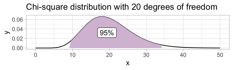
Example 8.5: Construct CI from pivot
We are modeling breakdowns in an insulating fluid between electrodes as \(X\sim Exponential(\lambda)\). A sample \(\boldsymbol{x}=[39.667, 132.179, 56.698, 7.638, 94.635, 292.725, 62.797, 82.026, 238.32, 142.972]\) with 10 observations has been collected. We want a 95% CI for \(\lambda\) and a 95% CI for the average breakdown time.
We found the pivot \(2\lambda\sum X_i\sim\chi^2(2n)\).
We can compute \(\sum X_i = 39.667 + 132.179 + 56.698 + 7.638 + 94.635 + 292.725 + 62.797 + 82.026 + 238.32 + 142.972 = 1149.657\).
With the quantile method (pick \(CDF^{-1}(\alpha/2)\) and \(CDF^{-1}(1-\alpha/2)\)) of creating a CI, this produces: \[ \begin{align*} CDF^{-1}_{\chi^2(5)}(0.025) \approx 9.59 &\leq 2\lambda\sum X_i & 2\lambda\sum X_i &\leq 34.17 \approx CDF^{-1}_{\chi^2(5)}(0.975) \\ \frac{9.59}{2\cdot 1149.657} \approx 0 &\leq \lambda & \lambda &\leq 0.0148608 \approx \frac{34.1696069}{2\cdot 1149.657} \end{align*} \]
We also produce, from the same pivot expressions: \[ \begin{align*} 9.59 &\leq 2\lambda\sum X_i & 2\lambda\sum X_i &\leq 34.17 \\ \EE[X] = \frac{1}{\lambda} &\leq \color{Teal}{\frac{2\sum X_i}{9.59}} & \color{SlateBlue}{\frac{2\sum X_i}{34.17}} &\leq \frac{1}{\lambda} = \EE[X] \\ \color{SlateBlue}{67.2912043} &\leq \EE[X] & \EE[X] &\leq \color{Teal}{239.7421925} \end{align*} \]
Gamma, Exponential and \(\chi^2\) - MGFs
We can look up the Moment Generating Functions for \(Gamma(k,\theta)\), for \(Exponential(\lambda)\) and for \(\chi^2(\nu)\):
| \(Exponential(\lambda)\) | \(\chi^2(\nu)\) | \(Gamma(k,\theta)\) | |
|---|---|---|---|
| MGF | \(\frac{\lambda}{\lambda-t} = \frac{1}{1-t/\lambda}\) | \(\frac{1}{(1-2t)^{\nu/2}}\) | \(\frac{1}{(1-\theta t)^k}\) |
By matching like with like, and using that equal MGF implies equal distributions, we see that
- \(Exponential(\lambda) = Gamma(1, 1/\lambda)\)
- \(\chi^2(\nu) = Gamma(\nu/2, 2)\)
It is a fact about MGFs that \(M_{\sum a_i X_i}(t) = \prod M_{X_i}(a_i t)\) (follows quickly from the definition of \(M_X(t) = \EE[e^{tX}]\)). Applied to a collection of \(X_i\sim Gamma(k_i, \theta)\) variables, we get
\[ M_{\sum X_i}(t) = \prod M_{X_i}(t) = \prod\frac{1}{(1-\theta t)^{k_i}} = \frac{1}{(1-\theta t)^{\sum k_i}} \]
Which is the MGF of a \(Gamma(\sum k_i, \theta)\) variable.
Finally, for \(M_{cX}(t) = \EE[e^{t\cdot cX}] = \EE[e^{tc\cdot X}] = M_{X}(ct)\). For the case of \(X\sim Gamma(k,\theta)\), we have \[ M_{cX}(t) = M_X(ct) = \frac{1}{(1-\theta\cdot ct)^k} = \frac{1}{(1-\theta c\cdot t)^k} \]
Which is the MGF of a \(\Gamma(k, c\theta)\) variable.
Interpreting Confidence Intervals
Practical statistics is plagued with subtle differences in interpretation and commonly occurring erroneous interpretations.
The confidence level of a confidence interval is the frequentist probability that the interval contain the true value. This is a statement about random variables.
Writing \(L=L(\boldsymbol{X})\) and \(U=U(\boldsymbol{X})\) for the lower and upper bounds as statistics for a sample \(\boldsymbol{X}=X_1,\dots,X_n\sim\mathcal{D}(\theta)\) iid, the confidence level measures \(\PP(L\leq \theta \leq U)\)
Once you have an observation \(\boldsymbol{x}=x_1,\dots,x_n\), there is nothing random about the process - the corresponding confidence interval is uniquely determined by the data. Writing similarly \(l=l(\boldsymbol{x})\) and \(u=u(\boldsymbol{x})\), there is nothing random about a claim \(l\leq\theta\leq u\) - it is either true or not true, and we will usually not be able to tell. \(\PP(l\leq\theta\leq u)\) can be generously interpreted as taking on either the value \(0\) or \(1\) depending on the true value of \(\theta\) - or otherwise is meaningless as a statement.
What the probabilistic statement of confidence levels does say is - like with all frequentist probability - that if the entire process (draw a random sample, compute confidence intervals, check whether \(L\leq\theta\leq U\)) is repeated a large number of times, then the proportion of resulting \((L,U)\) intervals that do contain \(\theta\) approaches the confidence level \(1-\alpha\).
Example - \(Exponential(\lambda)\)
Recall we derived the Confidence Interval for \(\EE[X] = \frac{1}{\lambda}\): \[ \frac{2\sum X_i}{34.17} \leq \frac{1}{\lambda} \leq \frac{2\sum X_i}{9.59} \]
Code
df = tibble(x=1:100, y=Xs, ylo=2*y/qchisq(0.975,20), yhi=2*y/qchisq(0.025,20), ymid=2*y/qchisq(0.5,20), contains=(ylo<EX) & (EX<yhi))
df %>%
  ggplot(aes(y=x)) +
  geom_pointrangeh(aes(x=y/10, xmin=ylo, xmax=yhi, color=contains), size=0.1) +
  geom_vline(xintercept=EX, color="thistle", size=1) +
  scale_color_discrete(type=c("#E69F00", "#56B4E9")) +
  guides(color="none") +
  labs(title="Confidence intervals for EX", subtitle="Middle dot indicates sample mean") +
  theme_light()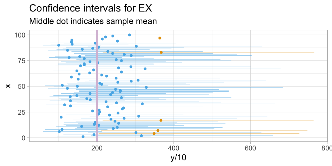
Out of 100 samples drawn and CIs computed from the random samples, 95 contain the target expected value.
Long term probability of accuracy
Exercise 8.11: Consider 1000 CIs for the distribution mean \(\mu\) at level 95%, drawn from independent data sets.
- How many of these do you expect to capture the corresponding value of \(\mu\)?
95% of 1000 is 950 - we would expect on average to capture the correct value 950 times.
- \(\PP(940 \leq \text{# correct intervals} \leq 960)\)?
The # of correct intervals is a Binomial variable: \(Y = Binomial(1000, 0.95)\). So we can compute the corresponding probability. In order to include \(940\) in the range we need to subtract \(CDF(939)\) and not \(CDF(940)\):
Four CIs for binomial probabilities
Let \(X\sim Binomial(n,p)\) be a single observation, \(n\) known. The MLE for \(p\) is \(\hat{p}=X/n\). We would like to construct a Confidence Interval for \(p\).
Difficulty There is no obvious pivotal quantity to work with here.
Say, for a running example, that we draw \(X\sim Binomial(200,p)\) and observe \(x=34\).
One way to think about the confidence interval \((L,U)\) is that given a specific observation \(X\), \(L\) is the smallest parameter value so that the upper and lower tails are not bigger than \(\alpha/2\) each, and \(U\) is the largest parameter value so that the upper and lower tails are not bigger than \(\alpha/2\) each.
Focusing on the tail that would be heavier in each case, this means for the binomial case finding \(p_L\) and \(p_U\) such that: \[ p_L = \arg\max \{p_L : 1-CDF_{Binomial(n,p_L)}(x) == 0.025 \} \qquad p_U = \arg\max \{p_U : CDF_{Binomial(n,p_U)}(x) == 0.025 \} \]
These equations are not easily solved algebraically - instead we take numeric approaches.
Four CIs for binomial probabilities
Let \(X\sim Binomial(n,p)\) be a single observation, \(n\) known. The MLE for \(p\) is \(\hat{p}=X/n\). We would like to construct a Confidence Interval for \(p\).
Difficulty There is no obvious pivotal quantity to work with here.
Say, for a running example, that we draw \(X\sim Binomial(200,p)\) and observe \(x=34\).
Now, suppose instead that since \(n\) is large we use an approximating distribution. If \(X\sim Binomial(n,p)\), then \(X\sim I_1+\dots+I_m\) where the \(I_k\) are iid Bernoulli variables indicating individual success experiments.
Since we are summing up iid variables, with \(\EE=p\) and \(\VV=p(1-p)\), the Central Limit Theorem applies, and we get:
\[ \frac{X-np}{\sqrt{np(1-p)}} \sim \mathcal{N}(0,1) \]
This can absolutely be used as a pivotal quantity, and we get with \(\PP=0.95\) that \(-1.96 \leq \frac{X-np}{\sqrt{np(1-p)}} \leq 1.96\). To solve for \(p\), we will need to get rid of the square root - so square all sides and we get:
\[ \begin{align*} \frac{(X-np)^2}{np(1-p)} &\leq 1.96^2 \\ (X-np)^2 - 1.96^2np(1-p) & \leq 0 \\ n^2p^2-2npX+X^2 - 1.96^2np+1.96^2np^2 &\leq 0 \\ (n^2+1.96^2n)p^2 + (-2Xn-1.96^2n)p + X^2 \leq 0 \end{align*} \]
Since \(n^2+1.96^2n\geq 0\), the quadratic will be negative between the two real roots. Solving the quadratic for \(p\) we get the roots \[ \begin{align*} p_L &= \frac{2Xn+1.96^2n-\sqrt{(2Xn+1.96^2n)^2-4(n^2+1.96^2n)X^2}}{2(n^2+1.96^2n)} \\ p_U &= \frac{2Xn+1.96^2n-\sqrt{(2Xn+1.96^2n)^2-4(n^2+1.96^2n)X^2}}{2(n^2+1.96^2n)} \end{align*} \]
For our running example, with \(n=200\) and \(X=34\) we get the interval (\(0.1243\), \(0.2282\))
Four CIs for binomial probabilities
Let \(X\sim Binomial(n,p)\) be a single observation, \(n\) known. The MLE for \(p\) is \(\hat{p}=X/n\). We would like to construct a Confidence Interval for \(p\).
Difficulty There is no obvious pivotal quantity to work with here.
Say, for a running example, that we draw \(X\sim Binomial(200,p)\) and observe \(x=34\).
The algebra got really messy there, largely because we had \(p\) in both numerator and denominator of our pivot.
Instead, we can use \(\hat{p} = X/n\), and write \[ \frac{\hat{p}-p}{\sqrt{\frac{\hat{p}(1-\hat{p})}{n}}} \sim \mathcal{N}(0,1) \]
With this pivot, we get \[ \begin{align*} -1.96 &\leq \frac{\hat{p}-p}{\sqrt{\frac{\hat{p}(1-\hat{p})}{n}}} & \frac{\hat{p}-p}{\sqrt{\frac{\hat{p}(1-\hat{p})}{n}}} & \leq 1.96 \\ \color{Teal}{-\hat{p}-1.96\sqrt{\frac{\hat{p}(1-\hat{p})}{n}}} &\leq -p & -p &\leq \color{DarkGoldenrod}{-\hat{p}+1.96\sqrt{\frac{\hat{p}(1-\hat{p})}{n}}} \\ \color{DarkGoldenrod}{\hat{p}-1.96\sqrt{\frac{\hat{p}(1-\hat{p})}{n}}} &\leq p & p & \leq \color{Teal}{\hat{p}+1.96\sqrt{\frac{\hat{p}(1-\hat{p})}{n}}} \end{align*} \]
This produces the interval: \(( 0.1179409, 0.2220591 )\)
Four CIs for binomial probabilities
Let \(X\sim Binomial(n,p)\) be a single observation, \(n\) known. The MLE for \(p\) is \(\hat{p}=X/n\). We would like to construct a Confidence Interval for \(p\).
Difficulty There is no obvious pivotal quantity to work with here.
Say, for a running example, that we draw \(X\sim Binomial(200,p)\) and observe \(x=34\).
Finally, since \(X/n\) is an MLE, we can use the sampling distribution of MLEs to build a confidence interval.
We proved using Cramér-Rao that the limiting distribution of \(\sqrt{n}(\hat\theta-\theta)\) is \(\mathcal{N}(0,1/\mathcal{I}(\theta))\). Hence
\[ \frac{\hat{p}-p}{\frac{1}{\sqrt{n}}\sqrt{\frac{1}{\mathcal{I}(p)}}} \sim \mathcal{N}(0,1) \qquad\text{and notice}\qquad \frac{\hat{p}-p}{\frac{1}{\sqrt{n}}\sqrt{\frac{1}{\mathcal{I}(p)}}} = \frac{\hat{p}-p}{\sqrt{\frac{p(1-p)}{n}}} \]
We can use this as a pivot!
\[ \begin{align*} -1.96 &\leq \frac{\hat{p}-p}{\sqrt{\frac{p(1-p)}{n}}} & \frac{\hat{p}-p}{\sqrt{\frac{p(1-p)}{n}}} &\leq 1.96 \end{align*} \]
This produces the exact same confidence interval as the previous slide, but with a different derivation.
Four CIs for binomial probabilities
Let \(X\sim Binomial(n,p)\) be a single observation, \(n\) known. The MLE for \(p\) is \(\hat{p}=X/n\). We would like to construct a Confidence Interval for \(p\).
Four constructions gave us three different options:
- \((0.125, 0.2294)\) with width \(0.1043\)
- \((0.1243\), \(0.2282)\) with width \(0.1039\) - but only for large enough samples
- \(( 0.1179, 0.2221 )\) with width \(0.1041\) - but only for large enough samples
A Confidence Interval for \(\mu\)
Suppose \(X_1,\dots,X_n\sim\mathcal{N}(\mu,\sigma^2)\), and suppose that \(\sigma^2\) is known. We can use the pivot method to construct a confidence interval:
\[ \begin{align*} \overline{X} &\sim\mathcal{N}(\mu,\sigma^2/n) \\ \overline{X}-\mu &\sim\mathcal{N}(0,\sigma^2/n) \\ \frac{\overline{X}-\mu}{\sigma/\sqrt{n}} &\sim\mathcal{N}(0,1) \end{align*} \]
Write \(z_{\alpha/2} = CDF^{-1}(1-\alpha/2)\) and note that because \(\mathcal{N}(0,1)\) is symmetric around 0, \(CDF^{-1}(\alpha/2) = -z_{\alpha/2}\). \[ \begin{align*} -z_{\alpha/2} &\leq \frac{\overline{X}-\mu}{\sigma/\sqrt{n}} & \frac{\overline{X}-\mu}{\sigma/\sqrt{n}} &\leq z_{\alpha/2} \\ -z_{\alpha/2}\sigma/\sqrt{n} &\leq \overline{X}-\mu & \overline{X}-\mu &\leq z_{\alpha/2}\sigma/\sqrt{n} \\ -\overline{X}-z_{\alpha/2}\sigma/\sqrt{n} &\leq -\mu & -\mu &\leq -\overline{X} + z_{\alpha/2}\sigma/\sqrt{n} \\ \overline{X}+z_{\alpha/2}\sigma/\sqrt{n}&\geq \mu & \mu &\geq \overline{X}-z_{\alpha/2}\sigma/\sqrt{n} \end{align*} \]
We get a confidence interval for \(\mu\) as \((\overline{X}-z_{\alpha/2}\sigma/\sqrt{n}, \overline{X}+z_{\alpha/2}\sigma/\sqrt{n})\).
A Confidence Interval for \(\mu\)
Suppose \(X_1,\dots,X_n\sim\mathcal{N}(\mu,\sigma^2)\), and suppose that \(\sigma^2\) is not known. We will have to estimate \(\sigma^2\), and we already know \(S^2 = \frac{1}{n-1}\sum(X_i-\overline{X})^2\) to be an unbiased consistent estimator. Hence, with large enough \(n\), \(\sigma^2\approx S^2\). (large enough: \(n>40\))
Following the same derivation as the previous slide, we can conclude that:
Theorem
If \(n\) is sufficiently large, and for any distribution for which the Central Limit Theorem holds, the standardized variable \[ Z = \frac{\overline{X}-\mu}{S/\sqrt{n}} \overset{\approx}{\sim}\mathcal{N}(0,1) \] so that \(Z\) works as a pivot. This implies that
\[ \overline{x}\pm z_{\alpha/2}s/\sqrt{n} \] is a large sample confidence interval for \(\mu\) with confidence level approximately \(1-\alpha\).
Wald’s Confidence Interval - CI for any \(\hat\theta\)
We have seen several confidence intervals now that follow the exact same pattern:
- \(p \in \hat{p}\pm z_{\alpha/2}\sqrt{\frac{\hat{p}(1-\hat{p})}{n}}\) (for large \(n\))
- \(\mu \in \overline{x}\pm z_{\alpha/2}\sigma/\sqrt{n}\) (for known \(\sigma^2\))
- \(\mu \in \overline{x}\pm z_{\alpha/2}s/\sqrt{n}\) (for large \(n\))
The fact used in all these three cases was that we had an estimator \(\hat\theta\) of a quantity \(\theta\) such that:
- \(\hat\theta\overset{\approx}{\sim}\mathcal{N}(\theta, \sigma^2_{\hat\theta})\)
- \(\hat\theta\) is (approximately) unbiased
- We know how to estimate \(\sigma_{\hat\theta}\).
In such a situation, we can conclude \(\frac{\hat\theta-\theta}{\sigma_{\hat\theta}}\sim\mathcal{N}(0,1)\) is a pivot:
\[ \begin{align*} -z_{\alpha/2} &\leq \frac{\hat\theta-\theta}{\sigma_{\hat\theta}} & \frac{\hat\theta-\theta}{\sigma_{\hat\theta}} &\leq z_{\alpha/2} \\ -z_{\alpha/2}\sigma_{\hat\theta} &\leq \hat\theta-\theta & \hat\theta-\theta &\leq z_{\alpha/2}\sigma_{\hat\theta} \\ \hat\theta+z_{\alpha/2}\sigma_{\hat\theta} &\geq \theta & \theta &\geq \hat\theta - z_{\alpha/2}\sigma_{\hat\theta} \end{align*} \]
The resulting CI \(\hat\theta\pm z_{\alpha/2}\sigma_{\hat\theta}\) or its estimated large(r) sample equivalent \(\hat\theta\pm z_{\alpha/2}s_{\hat\theta}\) is closely related to a generic hypothesis test construction by Wald.
Binomial Confidence Intervals revisited
With the Wald approach, we can get the pivot expression \(\frac{\hat{p}-p}{\sqrt{p(1-p)/n}}\). This we used last lecture with an approximation of \(p\) in the denominator. Writing \(q=1-p, \hat{q}=1-\hat{p}\), we can square the inequalities to get
\[ \begin{align*} \frac{{p}^2 - 2\hat{p}p + \hat{p}^2}{p(1-p)/n} &\leq z_{\alpha/2}^2 \\ {p}^2-2\hat{p}p+\hat{p}^2 &\leq z_{\alpha/2}^2 p/n - z_{\alpha/2}p^2/n \\ \color{Teal}{(1+z_{\alpha/2}^2/n)}p^2 - \color{DarkGoldenrod}{(2\hat{p}+z_{\alpha/2}^2/n)}p + \color{DarkMagenta}{\hat{p}^2} &\leq 0 \end{align*} \]
Solving the quadratic for \(p\) yields us the endpoints of the interval:
\[ p= \frac{\color{DarkGoldenrod}{-b}\pm\sqrt{\color{DarkGoldenrod}{b}^2-4\color{Teal}{a}\color{DarkMagenta}{c}}}{2\color{Teal}{a}} = \frac{\color{DarkGoldenrod}{(2\hat{p}+z_{\alpha/2}^2/n)}\pm\sqrt{\color{DarkGoldenrod}{(2\hat{p}+z_{\alpha/2}^2/n)}^2-4\color{Teal}{(1+z_{\alpha/2}^2/n)}\color{DarkMagenta}{\hat{p}^2}}}{2\color{Teal}{(1+z_{\alpha/2}^2/n)}} = \\ = \frac{\hat{p}+z_{\alpha/2}^2/(2n)}{1+z_{\alpha/2}^2/n} \pm\frac{\sqrt{\color{Teal}{4\hat{p}^2}+4\hat{p}z_{\alpha/2}^2/n+z_{\alpha/2}^4/n^2 \color{Teal}{- 4\hat{p}^2}-4\hat{p}^2 z_{\alpha/2}^2/n}}{2(1+z_{\alpha/2}^2/n)} = \\ = \frac{\hat{p}+z_{\alpha/2}^2/(2n)}{1+z_{\alpha/2}^2/n} \pm\frac{2z_{\alpha/2}\sqrt{\hat{p}/n - \hat{p}^2/n + z_{\alpha/2}^2/(4n^2)}}{2(1+z_{\alpha/2}^2/n)} = \\ = \frac{\hat{p}+z_{\alpha/2}^2/(2n)}{1+z_{\alpha/2}^2/n} \pm z_{\alpha/2}\frac{\sqrt{\hat{p}\hat{q}/n+z_{\alpha/2}^2/(4n^2)}}{1+z_{\alpha/2}^2/n} \]
This is called the score Confidence Interval for \(p\).
Large sample score CI for \(p\)
\[ p\in \frac{\hat{p}+\color{DarkMagenta}{z_{\alpha/2}^2/(2n)}}{1+\color{DarkMagenta}{z_{\alpha/2}^2/n}} \pm z_{\alpha/2}\frac{\sqrt{\hat{p}\hat{q}/n+\color{DarkMagenta}{z_{\alpha/2}^2/(4n^2)}}}{1+\color{DarkMagenta}{z_{\alpha/2}^2/n}} \]
As \(n\) grows large, \(z_{\alpha/2}^2/(2n)\approx0\), \(z_{\alpha/2}^2/n\approx0\) and \(z_{\alpha/2}^2/(4n^2)\approx0\), leaving the large sample CI
\[ p\in\hat p\pm z_{\alpha/2}\sqrt{\hat p\hat q/n} \]
Experiment: how often does the CI cover \(p\)?
We have several CIs for \(p\) now:
- \(p\in\hat p\pm z_{\alpha/2}\sqrt{\hat p\hat q/n}\)
- \(p\in \frac{\hat{p}+{z_{\alpha/2}^2/(2n)}}{1+{z_{\alpha/2}^2/n}} \pm z_{\alpha/2}\frac{\sqrt{\hat{p}\hat{q}/n+{z_{\alpha/2}^2/(4n^2)}}}{1+{z_{\alpha/2}^2/n}}\)
- \(p\in(L,U)\) where \(L,U\) are found by a root finder and the \(CDF^{-1}\).
This code block goes through values of \(p\) from \(0\) to \(1\), and for each, it generates 100 samples of \(100\) binomial values each, and computes these three confidence intervals for each sample and checks whether \(p\) is in the resulting interval.
Code
import scipy as sp
import numpy as np
from scipy.stats import binom, norm
from scipy.optimize import fsolve
N = 100
Nx = 100
Np = 101
alpha = 0.05
def phat(x): return x/N
def qhat(x): return phat(N-x)
def CI1(x): return {
  "lo": phat(x)+norm.ppf(alpha/2)*np.sqrt(phat(x)*qhat(x)/N),
  "hi": phat(x)+norm.isf(alpha/2)*np.sqrt(phat(x)*qhat(x)/N)
}
def CI2(x):
  za22 = norm.isf(alpha/2)**2
  return {
  "lo": (phat(x)+za22/(2*N))/(1+za22/N) + norm.ppf(alpha/2)*np.sqrt(phat(x)*qhat(x)/N + za22/(4*N**2))/(1+za22/N),
  "hi": (phat(x)+za22/(2*N))/(1+za22/N) + norm.isf(alpha/2)*np.sqrt(phat(x)*qhat(x)/N + za22/(4*N**2))/(1+za22/N)
}
def CI3(x):
  def pLopt(p_cand):
    return binom.sf(x,n=N,p=p_cand) - 0.025
  def pUopt(p_cand):
    return binom.cdf(x,n=N,p=p_cand) - 0.025
  return {"lo": fsolve(pLopt, x/N)[0], "hi": fsolve(pUopt, x/N)[0] }

def pInCI(p,CI): return (CI["lo"]<=p) and (p<=CI["hi"])
ps = np.linspace(0,1,Np)

experiments = np.array([[(p,pInCI(p, CI1(x)), pInCI(p, CI2(x)), pInCI(p, CI3(x))) for x in binom.rvs(N,p,size=Nx)] for p in ps]).sum(axis=1)
/opt/homebrew/lib/python3.10/site-packages/scipy/optimize/_minpack_py.py:175: RuntimeWarning:
The iteration is not making good progress, as measured by the
improvement from the last ten iterations.(I had to try 5 times to get the code for the 2nd CI correct)
Experiment: how often does the CI cover \(p\)?
We have several CIs for \(p\) now:
- \(p\in\hat p\pm z_{\alpha/2}\sqrt{\hat p\hat q/n}\)
- \(p\in \frac{\hat{p}+{z_{\alpha/2}^2/(2n)}}{1+{z_{\alpha/2}^2/n}} \pm z_{\alpha/2}\frac{\sqrt{\hat{p}\hat{q}/n+{z_{\alpha/2}^2/(4n^2)}}}{1+{z_{\alpha/2}^2/n}}\)
- \(p\in(L,U)\) where \(L,U\) are found by a root finder and the \(CDF^{-1}\).
Code
library(tidyverse)
library(reticulate)
experiments = tibble(
  ps = py$ps,
  CI1 = py$experiments[,2],
  CI2 = py$experiments[,3],
  CI3 = py$experiments[,4]
) %>% pivot_longer(c(CI1,CI2,CI3))
ggplot(experiments, aes(x=ps, y=value)) +
  geom_line(aes(color=name)) +
  xlab("p") + ylab("P(p in CI)") +
  labs(title="Coverage probability for 3 Confidence Intervals")