Estimators: Information, Efficiency
\[
\def\RR{{\mathbb{R}}}
\def\PP{{\mathbb{P}}}
\def\EE{{\mathbb{E}}}
\def\VV{{\mathbb{V}}}
\]
Example: Bernoulli
Let \(X\sim Bernoulli(p)\), with \(PDF(x|p) = p^x(1-p)^{1-x}\).
\[
\frac{d}{dp}\log(PDF(X|p)) =
\frac{d}{dp}\left(X\log p + (1-X)\log(1-p)\right) =
\frac{X}{p} - \frac{1-X}{1-p} = \frac{X-p}{p(1-p)} \\
\mathcal{I}(p) = \VV\left[\frac{d}{dp}\log(PDF(X|p))\right] =
\VV\left[\frac{X-p}{p(1-p)}\right] =
\frac{\VV[X]}{(p(1-p))^2} = \frac{p(1-p)}{(p(1-p))^2} = \frac{1}{p(1-p)}
\]
Alternatively
\[
\frac{d^2}{dp^2}\log(PDF(X|p)) =
\frac{d}{dp}\left(\frac{X}{p}-\frac{1-X}{1-p}\right) =
-\frac{X}{p^2}-\frac{1-X}{(1-p)^2} \\
\mathcal{I}(p) =
-\EE\left[\frac{d^2}{dp^2}\log(PDF(X|p))\right] =
\frac{p}{p^2}+\frac{1-p}{(1-p)^2} = \frac{1}{p}+\frac{1}{1-p} = \frac{1}{p(1-p)}
\]
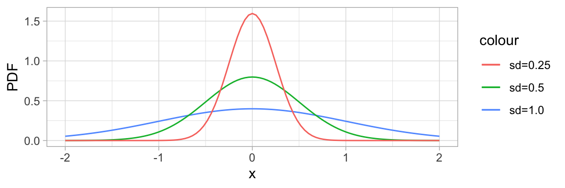
Example: Normal, known variance
As in our first motivating example, let \(X\sim\mathcal{N}(\mu,\sigma^2)\) with known \(\sigma^2\).
The score is: \[
\frac{d}{d\mu}\log(PDF(x | \mu,\sigma^2)) =
\frac{d}{d\mu}\left(-\log(\sqrt{2\pi\sigma^2}) - \frac{1}{2\sigma^2}(x-\mu)^2\right) =
\frac{1}{\sigma^2}(x-\mu)
\]
So the Fisher information is: \[
\mathcal{I}(\mu) =
\VV\left[\frac{1}{\sigma^2}(x-\mu)\right] =
\EE\left[\left(\frac{1}{\sigma^2}(x-\mu)\right)^2\right] =
\frac{1}{\sigma^4}\EE[(x-\mu)^2] =
\frac{1}{\sigma^4}\VV[x] =
\frac{\sigma^2}{\sigma^4} = \frac{1}{\sigma^2}
\]
Just like we set out for our information measure to be in the initial motivating example.
Cramér-Rao: How good can an estimator get?
Harald Cramér in Sweden and CR Rao in India independently derived this lower bound based on Fisher information:
Let \(X_1,\dots,X_n\sim\mathcal{D}(\theta)\) iid where the support1 does not depend on \(\theta\). If the statistic \(T=t(X_1,\dots,X_n)\) is an unbiased estimator for \(\theta\), then
\[
\VV[T] \geq \frac{1}{\mathcal{I}_n(\theta)}
\]
Proof
Consider the covariance \(Cov(T, \ell'(\theta))\) of the estimator with the score function.
\[
Cov(T(\boldsymbol{x}), \ell'(\theta|\boldsymbol{x})) =
\EE[T(\boldsymbol{x})\cdot\ell'(\theta|\boldsymbol{x})] - \EE[T(\boldsymbol{x})]\cdot\EE[\ell'(\theta|\boldsymbol{x})] =
\EE[T(\boldsymbol{x})\cdot\ell'(\theta|\boldsymbol{x})] \\
\begin{align*}
\EE[T(\boldsymbol{x})\cdot\ell'(\theta|\boldsymbol{x})] &=
\iiint T(x_1,\dots,x_n)\cdot\ell'(\theta|\boldsymbol{x})PDF(x_1,\dots,x_n|\theta)dx_1\dots dx_n \\
&= \iiint
T(x_1,\dots,x_n)\cdot
\left(\frac{\frac{d}{d\theta}PDF(x_1,\dots,x_n|\theta)}
{\color{DarkRed}{PDF(x_1,\dots,x_n|\theta)}}
\right)
\color{DarkRed}{PDF(x_1,\dots,x_n|\theta)}
dx_1\dots dx_n \\
&= \iiint T(x_1,\dots,x_n)\frac{d}{d\theta}PDF(x_1,\dots,x_n|\theta)dx_1\dots dx_n \\
&= \frac{d}{d\theta}\iiint T(x_1,\dots,x_n) PDF(x_1,\dots,x_n|\theta) dx_1\dots dx_n \\
&= \frac{d}{d\theta}\EE[T(\boldsymbol{x})] = \frac{d}{d\theta}\theta = 1
\end{align*}
\]
Cramér-Rao: How good can an estimator get?
Harald Cramér in Sweden and CR Rao in India independently derived this lower bound based on Fisher information:
Let \(X_1,\dots,X_n\sim\mathcal{D}(\theta)\) iid where the support1 does not depend on \(\theta\). If the statistic \(T=t(X_1,\dots,X_n)\) is an unbiased estimator for \(\theta\), then
\[
\VV[T] \geq \frac{1}{\mathcal{I}_n(\theta)}
\]
Proof (cont…)
We established \(Cov(T, \ell') = \EE[T(\boldsymbol{x})\cdot\ell'(\theta|\boldsymbol{x})] = 1\).
Covariance is connected to the correlation \(\rho\) through \(\rho(X,Y) = \frac{Cov(X,Y)}{\sigma_X\sigma_Y}\). Remember that the correlation coefficient is bound by \(\pm1\) so that \(-1\leq\rho\leq1\). Squaring this, we get
\[
1 \geq \rho(T,\ell')^2 = \frac{Cov(T,\ell')^2}{\VV[T]\VV[\ell']} = \frac{1}{\VV[T]\VV[\ell']}
\]
Multiplying by \(\VV[T]\) and identifying \(\VV[\ell']=\mathcal{I}_n(\theta)\) finishes the proof.
Efficiency: How close are you to the Cramér-Rao lower bound?
The efficiency of an unbiased estimator \(T\) of a parameter \(\theta\) is the ratio \(\frac{1/\mathcal{I}_n(\theta)}{\VV[T]}\). An efficient estimator is one that achieves the Cramér-Rao lower bound, and is automatically an MVUE.
Example: Bernoulli
Let \(X_1,\dots,X_n\sim Bernoulli(p)\) iid. Our derivation earlier of \(\mathcal{I}(p)=\frac{1}{p(1-p)}\) tells us \(\mathcal{I}_n(p)=\frac{n}{p(1-p)}\).
Let \(T=\hat p=\overline{X}=\sum X_i/n\). This is an unbiased estimator, and \[
\VV[T] =
\VV\left[\sum X_i/n\right] =
\sum\frac{1}{n^2}\VV[X_i] = n\frac{p(1-p)}{n^2} = \frac{p(1-p)}{n} = \frac{1}{\mathcal{I}_n(p)}
\]
This proves that \(\hat{p}\) has efficiency \(1\), is an efficient estimator, and therefore is an MVUE.
Example: Normal
Let \(X_1,\dots,X_n\sim\mathcal{N}(\mu,\sigma^2)\) iid, with \(\sigma^2\) known. Our earlier derivation of \(\mathcal{I}(\mu)=\frac{1}{\sigma^2}\) tells us \(\mathcal{I}_n(\mu)=\frac{n}{\sigma^2}\).
Let \(T=\overline{X}\). This is an unbiased estimator, and \(\VV[T] = \frac{\sigma^2}{n} = \frac{1}{\mathcal{I}_n(\mu)}\), so \(\overline{X}\) is efficient and an MVUE.
Large Sample MLE
The Cramér-Rao lower bound helps us prove very nice properties for large sample MLE:
Let \(X_1,\dots,X_n\sim\mathcal{D}(\theta)\) iid, and assume that the set of possible values does not depend on \(\theta\).
Then for large \(n\), the sampling distribution of the MLE \(\hat\theta\) is approximately a normal distribution with mean \(\theta\) and variance \(1/(n\mathcal{I}(\theta))\).
The limiting distribution of \(\sqrt{n}(\hat\theta-\theta)\) is \(\mathcal{N}(0,1/\mathcal{I}(\theta))\).
Proof
The derivative of the score function \(U(\theta)=\frac{d}{d\theta}\ell(\theta)\) at the true \(\theta\) is approximately equal to the difference quotient \[
U'(\theta) \approx
\frac{U(\hat\theta)-U(\theta)}{\hat\theta-\theta}
\] Because \(\hat\theta\) is consistent, \(\hat\theta\to\theta\) as \(n\to\infty\). Because \(\hat\theta\) is the MLE, \(U(\hat\theta)=0\), and so in the limit: \[
\begin{align*}
\hat\theta-\theta &= \frac{U(\theta)}{-U'(\theta)} \\
\sqrt{n}(\hat\theta-\theta) &=
\frac{\sqrt{n}U(\theta)}{-U'(\theta)} =
\frac{(\sqrt{n}/(n\sqrt{\mathcal{I}(\theta))})U(\theta)}{-1/(n\sqrt{\mathcal{I}(\theta)}))} =
\frac{U(\theta)/\sqrt{n\mathcal{I}(\theta)}}{-(1/n)U'(\theta)/\sqrt{\mathcal{I}(\theta)}} \\
&= \frac
{\frac{1}{n}\left(\sum\frac{d}{d\theta}\log(PDF(X_i|\theta))\right)/\sqrt{\mathcal{I}(\theta)/n}}
{\frac{1}{n}\left(-\sum\frac{d^2}{d\theta^2}\log(PDF(X_i|\theta))\right)/\sqrt{\mathcal{I}(\theta)}}
\end{align*}
\]
Large Sample MLE
The Cramér-Rao lower bound helps us prove very nice properties for large sample MLE:
Let \(X_1,\dots,X_n\sim\mathcal{D}(\theta)\) iid, and assume that the set of possible values does not depend on \(\theta\).
Then for large \(n\), the sampling distribution of the MLE \(\hat\theta\) is approximately a normal distribution with mean \(\theta\) and variance \(1/(n\mathcal{I}(\theta))\).
The limiting distribution of \(\sqrt{n}(\hat\theta-\theta)\) is \(\mathcal{N}(0,1/\mathcal{I}(\theta))\).
Proof (cont…)
We established
\[
\sqrt{n}(\hat\theta-\theta) = \frac
{\frac{1}{n}\left(\sum\frac{d}{d\theta}\log(PDF(X_i|\theta))\right)/\sqrt{\mathcal{I}(\theta)/n}}
{\frac{1}{n}\left(-\sum\frac{d^2}{d\theta^2}\log(PDF(X_i|\theta))\right)/\sqrt{\mathcal{I}(\theta)}}
\]
Each \(\frac{d}{d\theta}\log(PDF(X_i|\theta))\) is an iid random variable with mean \(0\) and variance \(\mathcal{I}(\theta)\). The entire numerator is a z-score normalization, and by the central limit theorem is approximately \(\mathcal{N}(0,1)\).
Each \(-\frac{d^2}{d\theta^2}\log(PDF(X_i|\theta))\) is an iid random variable with mean \(\mathcal{I}(\theta)\). The whole denominator converges to \(\sqrt{\mathcal{I}(\theta)}\).
The ratio of a random variable distributed as \(\mathcal{N}(0,1)\) by the quantity \(\sqrt{\mathcal{I}(\theta)}\) is distributed as \(\mathcal{N}(0,1/\mathcal{I}(\theta))\). QED.
7.8 - Nicholas Basile
- \(\hat{p} = \frac{80-12}{80} = \frac{68}{80} = 0.85\) - 85% not defective.
- \(0.85\cdot 0.85 = 0.7225\) - two components - 72.25% of all systems that work properly.
- \[
\begin{align*}
\EE[\hat{p}^2] &= \VV[\hat{p}]+\EE[\hat{p}]^2 \\
\EE[\hat{p}] &= 0.85 \quad \text{by a.} \\
\VV[\hat{p}] &= \frac{p(1-p)}{n} = \frac{0.85\cdot0.15}{80}\approx 0.001 \\
\EE[\hat{p}^2] &\approx 0.001 + 0.85^2 \approx 0.7235
\EE[\hat{p}^2] &\neq p^2
\end{align*}
\] Because the variance is not 0, \(\EE[\hat{p}^2]\neq p^2\), therefore \(\hat{p}^2\) is biased.
7.10 - James Lopez
- \[
\begin{align*}
\EE[\overline{X}^2] &= \VV[\overline{X}] + \EE[\overline{X}]^2 \\
\VV[\overline{X}] &= \left(\frac{\sigma}{\sqrt{n}}\right)^2 = \frac{\sigma^2}{n} \\
\EE[\overline{X}]^2 &= \mu^2 \\
\EE[\overline{X}^2] &= \frac{\sigma^2}{n} + \mu^2 \\
\EE[\overline{X}^2] &\neq \mu^2 \qquad \text{so it is not unbiased.}
\end{align*}
\]
Since \(\EE[\overline{x}^2]\neq\mu^2\) not an unbiased estimator.
- \[
\begin{align*}
\EE[\overline{X}^2] &= \frac{\sigma^2}{n}+\mu^2 \\
\EE[S^2] &= \sigma^2 \\
\EE[\overline{X}^2-kS^2] &= \mu^2 \\
\frac{\sigma^2}{n}+\mu^2-k\sigma^2 &= \mu^2 \\
\frac{\sigma^2}{n} &= k\sigma^2 \\
\frac{1}{n} &= k
\end{align*}
\]
7.14 - Victoria Paukova
- If \(X_1=237, X_2=375, X_3=202, X_4=525, X_5=418\),
\[
\max(X_i)-\min(X_i)+1 = 525-202+1 = 324
\]
- The estimate will be exactly equal to the true value when the \(\max(X_i)\) actually corresponds to the first serial number and \(\min(X_i)\) corresponds to the last serial number. Since we know the serial numbers are an inclusive set, it’s not possible to overestimate the jet fighter amount. It is a biased estimator because it is very unlikely that \(\max(X_i)=\beta\) and \(\min(X_i)=\alpha\) in the sample.
7.21 a. - James Lopez
\(n=20\), \(x=3\), \(\log\) is base \(e\).
\[
\begin{align*}
\ell(p) &= \log\left[{n\choose x}p^x(1-p)^{n-x}\right] & \log ab &= \log a + \log b \\
&= \log{n\choose x}+x\log p + (n-x)\log(1-p) & \log a^x &= x\log a \\
\ell'(p) &= \frac{d}{dp}\left[\log{n\choose x}+x\log p+(n-x)\log(1-p)\right] \\
&= 0 + x\frac{1}{p}\cdot 1 + (n-x)\frac{1}{1-p}\cdot (-1) \\
&= \frac{x}{p} - \frac{n-x}{1-p} \\
\frac{x}{p}-\frac{n-x}{1-p} &= 0 \\
\frac{x}{p} &= \frac{n-x}{1-p} \\
x(1-p) &= p(n-x) \\
x-px &= pn-px \\
x &= pn \\
p = \frac{x}{n}
\end{align*}
\]
MLE of \(p\) is \(\hat{p} = \frac{x}{n} = \frac{3}{20} = 0.15\).
7.21 - James Lopez
- \[
\begin{align*}
\EE[\hat{p}] &= \EE\left[\frac{x}{n}\right] \\
&= \frac{1}{n}\EE[x]
\end{align*}
\]
For the binomial distribution, \(\EE[x] = np\).
\[
\begin{align*}
\EE[\hat{p}] &= \frac{1}{n}\cdot np \\
&= p
\end{align*}
\]
The estimator is unbiased.
- \[
\begin{align*}
(1-p)^5 &= (1-\hat{p})^5 \\
&= (1-0.15)^5 \\
&= 0.85^5 \\
&\approx 0.443705 \approx 0.444
\end{align*}
\]
7.24 - Maxim Kleyer
\[
\begin{align*}
f(x_1,\dots,x_n,y_1,\dots,y_n | \lambda_1,\lambda_2) &=
f(x_1|\lambda_1)\cdot\dots\cdot f(x_n|\lambda_1)\cdot
f(y_1|\lambda_2)\cdot\dots\cdot f(y_n|\lambda_2) = \\
&= \frac{e^{-n\lambda_1}\cdot\lambda_1^{\sum_{i=1}^nx_i}}{(x_1)!\cdot\dots\cdot(x_n!)}
\cdot
\frac{e^{-n\lambda_2}\cdot\lambda_2^{\sum_{i=1}^ny_i}}{(y_1)!\cdot\dots\cdot(y_n!)} = \\
&= \frac{e^{-n\lambda_1}\cdot\lambda_1^{n\overline{x}}}{(x_1)!\cdot\dots\cdot(x_n!)}
\cdot
\frac{e^{-n\lambda_2}\cdot\lambda_2^{n\overline{y}}}{(y_1)!\cdot\dots\cdot(y_n!)} \quad\text{ take log} \\
&= \ln(e^{-n\lambda_1}\cdot\lambda_1^{n\overline{x}}\cdot e^{-n\lambda_2}\cdot\lambda_2^{n\overline{y}}) - \ln((x_1!)\cdot\dots\cdot(x_n!)\cdot(y_1!)\cdot\dots\cdot(y_n!)) \\
&= n\overline{x}\ln\lambda_1 + n\overline{y}\ln\lambda_2 - n\lambda_1 - n\lambda_2 + [\dots] \quad\text{take }\frac{d}{d\lambda_1} \\
&= \frac{n\overline{x}}{\lambda_1} + 0 - n + 0 + 0 \Rightarrow \frac{n\overline{x}}{\lambda_1} - n = 0 \\
\end{align*} \\
\Rightarrow\boxed{\hat\lambda_1 = \overline{x}}
\]
Similarly \(\boxed{\hat\lambda_2=\overline{y}}\).
Now, \(\lambda_1-\lambda_2\Rightarrow\hat\lambda_1-\hat\lambda_2=\boxed{\overline{x}-\overline{y}}\).
7.25 - James Lopez
\[
\begin{align*}
\mathcal{L}(p) &= {x-1\choose r-1}p^r(1-p)^{x-r} \\
\ell(p) &= \log\left[{x-1\choose r-1}p^r(1-p)^{x-r}\right] \\
&= \log{x-1\choose r-1} + r\log(p) + (x-r)\log(1-p) \\
\ell'(p) &= \frac{d}{dp}\left[\log{x-1\choose r-1} + r\log(p) + (x-r)\log(1-p)\right] \\
&= 0 + \frac{r}{p}\cdot 1 + \frac{x-r}{1-p}\cdot(-1) = \frac{r}{p} - \frac{x-r}{1-p} \\
\end{align*}
\]
\[
\begin{align*}
0 &= \frac{r}{p} - \frac{x-r}{1-p} \\
\frac{x-r}{1-p} &= \frac{r}{p} \\
p(x-r) &= r(1-p) \\
xp-rp &= r-rp \\
xp &= r \\
p &= \frac{r}{x}
\end{align*}
\]
MLE of \(\hat{p} = \frac{r}{x} = \frac{3}{20} = 0.15\), which is the same MLE as 7.21.
In exercise 17, the unbiased estimator is \(\hat{p}=\frac{r-1}{x+r-1}=\frac{2}{19}\approx0.105263\) which is not the same.