Estimators: Methods for Point Estimators

Mikael Vejdemo-Johansson

\[ \def\RR{{\mathbb{R}}} \def\PP{{\mathbb{P}}} \def\EE{{\mathbb{E}}} \def\VV{{\mathbb{V}}} \]

Using sample moments to estimate parameters

Recall last lecture: using \(X_1,\dots,X_n\sim Uniform(0,\theta)\) we proposed using \(\hat\theta=2\overline{X}\) as an estimator, because \(\EE[X_i] = \theta/2\).

This is a first example of a generic approach:

Definition

Let \(X_1,\dots,X_n\sim\mathcal{D}\). The \(k\)th moment \(\mu_k=\EE[X^k]\). The \(k\)th sample moment is \(\frac{1}{n}\sum_i X_i^k\).

Suppose \(\mathcal{D}\) has a PMF/PDF with \(m\) parameters: \(f(x | \theta_1,\dots,\theta_m)\). The method of moment estimators \(\hat\theta_1,\dots,\hat\theta_m\) are obtained by equating the first \(m\) moments to their corresponding sample moments, and solving for \(\theta_1,\dots,\theta_m\)

Example: Uniform(a,b)

Let \(X_1,\dots,X_n\sim Uniform(a,b)\). We mean to estimate \(a\) and \(b\).

We know of the uniform distribution that \(\EE[X]=(a+b)/2\) and that \(\VV[X]=(b-a)^2/12\). So the method of moments approach calls on us to set up and solve:

\[ \begin{align*} \overline{X} &= \frac{\hat{a}+\hat{b}}{2} & S^2 &= \frac{(\hat{b}-\hat{a})^2}{12} \\ \hat{a} &= 2\overline{X}-\hat{b} & S^2 &= \frac{(\hat{b}-(2\overline{X}-\hat{b}))^2}{12} = \frac{(2\hat{b}-2\overline{X})^2}{12} \\ \hat{a} &= 2\overline{X}-\hat{b} & 12S^2 &= 4\hat{b}^2-4\hat{b}\overline{X}+4\overline{X}^2 \\ \hat{a} &= 2\overline{X}-\hat{b} & 0 &= \hat{b}^2-\hat{b}\overline{X}+\overline{X}^2-3S^2 \\ \hat{a} &= 2\overline{X}-\hat{b} & \hat{b} &= \frac{\overline{X}\pm\sqrt{\overline{X}^2-4(\overline{X}^2-3S^2)}}{2} = \frac{\overline{X}\pm\sqrt{3(S^2-\overline{X}^2)}}{2} \end{align*} \]

We can ignore the solution \(\hat{b}=(\overline{X}-\sqrt{3(S^2-\overline{X}^2)})/2\) because the upper limit is not smaller than the mean.

Maximum Likelihood Estimation

Another, far more popular method for creating estimators is the maximum likelihood estimator.

Definition

Given a distribution \(\mathcal{D}\) with some parameters \(\mathbf{\theta}\) and PDF \(f(\mathbf{x} | \mathbf{\theta})\) (where both \(\mathbf{x}=(x_1,\dots,x_n)\) and \(\mathbf{\theta}=(\theta_1,\dots,\theta_m)\) may be vectors), and an observed outcome \(x_1,\dots,x_n\sim\mathcal{D}\), the likelihood function \(\mathcal{L}(\mathbf{\theta}|\mathbf{x})\) is \(f\) viewed as a function of \(\mathbf{\theta}\).

The maximum likelihood estimator \(\hat\theta = \arg\max_{\mathbf{\theta}}\mathcal{L}(\mathbf{\theta}|\mathbf{x})\) is the values of \(\theta_1,\dots,\theta_n\) that maximize the likelihood function. We abbreviate it as MLE.

Since logarithms¹ are monotone, any maximum of \(\mathcal{L}\) is also a maximum of \(\log\mathcal{L}\). We often use \(\ell=\log\mathcal{L}\).

1. I will write \(\log\) even if the base is \(e\), and assume base \(e\) unless anything else is specified.

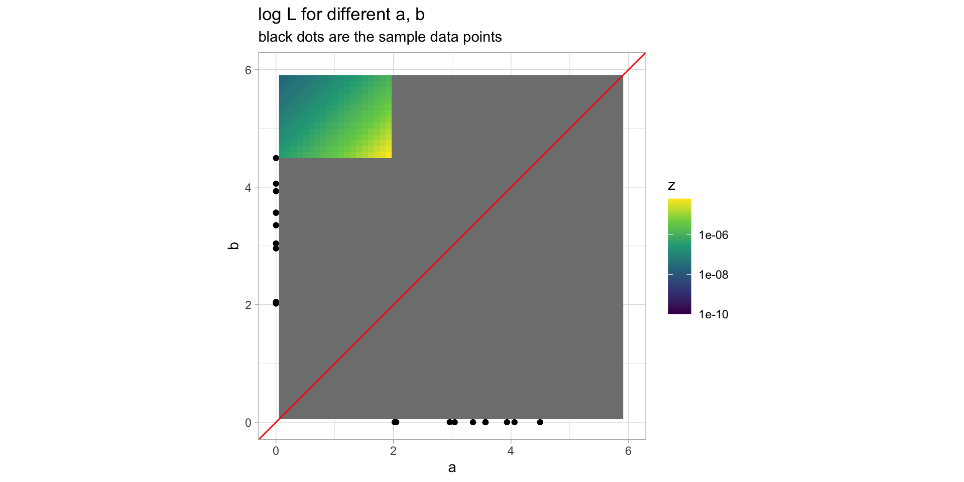
Example: Uniform(a,b)

Let \(X_1,\dots,X_n\sim Uniform(a,b)\). We mean to estimate \(a\) and \(b\).

We can write out the likelihood function:

\[ \mathcal{L}(a,b) = \begin{cases} 0 & \text{if } x_{(1)} < a \\ 0 & \text{if } x_{(n)} > b \\ \frac{1}{(b-a)^n} & \text{otherwise} \end{cases} \]

Code

library(tidyverse)

xs = runif(10, 2, 4.5)

L = function(a,b) {
  ifelse(a < min(xs), 
         ifelse(max(xs) < b,
                ifelse(a < b,
                      1/(b-a)^length(xs)
                      ,0)
                ,0)
         ,0)
}

gx = seq(0,10, length.out=100)
gy = seq(0,10, length.out=100)
gg = expand.grid(x=gx, y=gy) %>%
  mutate(z = L(x,y))

ggplot(gg, aes(x=x,y=y)) +
  geom_raster(aes(fill=z)) +
  scale_x_continuous(breaks=c(0,2,4,6), limits=c(0,6)) +
  scale_y_continuous(breaks=c(0,2,4,6), limits=c(0,6)) +
  scale_fill_viridis_c(trans="log10") +
  xlab("a") + ylab("b") + 
  labs(title="log L for different a, b", subtitle="black dots are the sample data points") +
  geom_abline(color="red") +
  geom_point(data=tibble(x=xs), aes(x=x, y=0)) +
  geom_point(data=tibble(x=xs), aes(x=0, y=x)) +
  coord_equal() +
  theme_light()

To maximize it, we need to look for critical points and boundary points.

\[ \begin{align*} \frac{d}{da}\frac{1}{(b-a)^n} &= \frac{n}{(b-a)^{n+1}} & \frac{d}{db}\frac{1}{(b-a)^n} &= \frac{-n}{(b-a)^{n+1}} \end{align*} \] This tells us there will be no critical points in the defined region.

So it remains to look along the boundary.

Example: Uniform(a,b)

Let \(X_1,\dots,X_n\sim Uniform(a,b)\). We mean to estimate \(a\) and \(b\).

\[ \mathcal{L}(a,b) = \begin{cases} 0 & \text{if } x_{(1)} < a \\ 0 & \text{if } x_{(n)} > b \\ \frac{1}{(b-a)^n} & \text{otherwise} \end{cases} \]

The boundary is the lines defined by \(b=\max x_i\) and \(a=\min x_i\). We may notice that the derivatives along these lines are:

\[ \begin{align*} \frac{d}{da}\mathcal{L}(a, \max x_i) &= \frac{n}{(\max x_i-a)^{n+1}} & \frac{d}{db}\mathcal{L}(\min x_i, b) &= \frac{-n}{(b-\min x_i)^{n+1}} \end{align*} \]

So the derivative along the horizontal boundary is always positive, and the derivative along the negative boundary is always negative. Neither is ever actually equal to 0.

The one remaining possible point for an extreme value is the point \((\min x_i, \max x_i)\), which turns out to actually hold the maximum likelihood.

Recall our \(Uniform(0,\theta)\) example

The two estimators we started with then were \(\theta=2\overline{X}\) and \(\theta=\max X\) - precisely the Method of Moments and the Maximum Likelihood estimators we just derived here.

Just like in the previous example, our MLE is biased and may need correction.

Another MLE: \(Exponential(\lambda)\)

Recall the exponential distribution: \(f(x|\lambda) = \lambda e^{-\lambda x}\). A random sample \(X_1,\dots,X_n\sim Exponential(\lambda)\) has joint likelihood function

\[ \begin{align*} \mathcal{L}(\lambda | x_1,\dots,x_n) &= (\lambda e^{-x_1\lambda})\cdot \dots \cdot(\lambda e^{-x_n\lambda}) = \lambda^n e^{-\lambda\sum x_i} \\ \ell(\lambda | x_1,\dots,x_n) &= \log\left(\lambda^n e^{-\lambda\sum x_i}\right) = n\log\lambda - \lambda\sum x_i \\ \end{align*} \]

We look for critical points and find \[ \begin{align*} \frac{d}{d\lambda}\ell(\lambda) &= \frac{n}{\lambda} - \sum x_i = 0 \\ \frac{n}{\lambda} &= \sum x_i \\ \lambda &= \frac{n}{\sum x_i} = \frac{1}{\overline{x}} \end{align*} \]

Another MLE: \(Normal(\mu,\sigma^2)\)

The joint density of \(X_1,\dots,X_n\sim\mathcal{N}(\mu,\sigma^2)\) is

\[ \begin{align*} f(\mathbf{x}|\mu,\sigma^2) = \mathcal{L}(\mu,\sigma^2) &= \left(\frac{1}{\sqrt{2\pi\sigma^2}}\right)^ne^{-\sum(x_i-\mu)^2/(2\sigma^2)} \\ \ell(\mu,\sigma^2) &= -\frac{n}{2}\log(2\pi\sigma^2) - \frac{1}{2\sigma^2}\sum(x_i-\mu)^2 \\ \frac{d}{d\mu}\ell(\mu,\sigma^2) &= -\frac{1}{2\sigma^2} \sum-2(x_i-\mu) = \frac{1}{\sigma^2}\left(\sum x_i - n\mu\right) \\ \frac{d}{d\sigma^2}\ell(\mu,\sigma^2) &= -\frac{n}{2}\frac{1}{2\pi\sigma^2}\cdot 2\pi - \frac{\sum(x_i-\mu)^2}{2}\cdot\frac{-1}{\sigma^4} = \frac{-n\sigma^2+\sum(x_i-\mu)^2}{2\sigma^4} \end{align*} \]

By multiplying by appropriate powers of \(\sigma^2\) (which is sure to be \(>0\)), the first equation yields \(\hat\mu=(\sum x_i)/n\) and the second equation yields \(\hat\sigma^2=(\sum(x_i-\mu)^2)/n\).

Another MLE: \(Poisson(\lambda)\)

Suppose \(X_1,\dots,X_n\sim Poisson(\lambda)\). Their joint PMF (and thus likelihood) is

\[ \begin{align*} p(\mathbf{x}|\lambda) = \mathcal{L}(\lambda) &= \frac{\lambda^{x_1}e^{-\lambda}}{x_1!}\cdot\dots\cdot\frac{\lambda^{x_n}e^{-\lambda}}{x_n!} = \frac{\lambda^{\sum x_i}e^{-n\lambda}}{x_1!\cdot\dots\cdot x_n!} \\ \ell(\lambda) &= \left(\sum x_i\right)\log\lambda - n\lambda - \sum\log(x_i!) \\ \frac{d}{d\lambda}\ell(\lambda) &= \frac{\sum x_i}{\lambda} - n \end{align*} \]

Which yields the estimator \(\hat\lambda = \overline{X}\).

Another MLE: Poisson Process

Suppose a region is subdivided into disjoint sample regions \(R_1,\dots,R_n\) and observations (eg counting plants of some fixed species) made so that \(X_1\sim Poisson(\lambda\cdot area(R_1)), \dots, X_n\sim Poisson(\lambda \cdot area(R_n))\).

The joint PMF/likelihood is:

\[ \begin{align*} p(\mathbf{x}|\lambda) = \mathcal{L}(\lambda) &= \frac{(\lambda\cdot area(R_1))^{x_1}e^{-\lambda\cdot area(R_1)}}{x_1!}\cdot\dots\cdot\frac{(\lambda\cdot area(R_n))^{x_n}e^{-\lambda\cdot area(R_n)}}{x_n!} \\ &= \frac{\lambda^{\sum x_i}\cdot\left(\prod area(R_i)^{x_i}\right)\cdot e^{-\lambda\cdot\sum area(R_i)}}{\prod x_i!} \\ \ell(\lambda) &= \log\lambda\cdot\sum x_i + \sum x_i\log(area(R_i)) - \lambda\sum area(R_i) - \sum\log(x_i!) \\ \frac{d}{d\lambda}\ell(\lambda) &= \frac{\sum x_i}{\lambda} - \sum area(R_i) \end{align*} \]

Finding the critical point yields our MLE \(\hat\lambda = (\sum x_i)/(\sum area(R_i))\).

Another MLE: Poisson Process through distance to nearest neighbor

Instead of counting quadrants (as the process on the previous slide is called), we could pick \(n\) points at random in the domain, and for each of them measure the distance to the nearest observation. Write \(y_i\) for this distance from the \(i\)th point to the nearest observation.

\[ \begin{multline*} CDF(y) = \PP(Y\leq y) = 1-\PP(Y > y) = \\ 1-\PP(\text{no plants in a circle of radius $y$}) \end{multline*} \]

With the point process from the previous slide, we can compute this probability: \[ \PP(Y > y) = PMF_{Poisson(\lambda\cdot area)}(0) = \frac{(\lambda\pi y^2)^0 e^{-\lambda\pi y^2}}{0!} \]

So \(CDF(y) = 1-e^{-\lambda\pi y^2}\), and \(PDF(y) = 2\pi\lambda ye^{-\lambda\pi y^2}\) for \(y\geq 0\).

Another MLE: Poisson Process through distance to nearest neighbor

We measure \(Y_i\), the distance to the nearest observation from the randomly chosen point \(x_i\). We have found \(CDF(y) = 1-e^{-\lambda\pi y^2}\), and \(PDF(y) = 2\pi\lambda ye^{-\lambda\pi y^2}\) for \(y\geq 0\).

We compute and differentiate the log likelihood: \[ \begin{align*} \mathcal{L}(\lambda | y_1,\dots,y_n) &= (2\pi\lambda)^n\cdot\left(\sum y_i\right)\cdot e^{-\lambda\pi\sum y_i^2} \\ \ell(\lambda | y_1,\dots,y_n) &= n\log(2\pi\lambda) + \log\left(\sum y_i\right) - \lambda\pi\sum y_i^2 \\ \frac{d}{d\lambda}\ell(\lambda | y_1,\dots,y_n) &= \frac{2\pi n}{2\pi\lambda} - \pi\sum y_i^2 = \frac{n}{\lambda}-\pi\sum y_i^2 \end{align*} \]

From this we get the MLE \(\hat\lambda = \frac{n}{\pi\sum y_i^2}\) or the ratio (number of plants observed)/(total area sampled).

Why we like MLEs - some properties that hold

Theorem

Let \(\hat\theta_1,\dots,\hat\theta_m\) be MLEs of the parameters \(\theta_1,\dots,\theta_m\).

Then the MLE of any function \(h(\theta_1,\dots,\theta_m)\) of these parameters is the function applied to the MLEs \(h(\hat\theta_1,\dots,\hat\theta_m)\).

We know the MLE for \(\sigma^2\) for a normal distribution - so we can directly write out the MLE for \(\sigma\):

\[ \hat\sigma = \sqrt{\frac{1}{n}\sum(X_i-\overline{X})^2} \]

It is, of course, a biased estimator. There are no guarantees that MLEs will be unbiased - and on top of that, Jensen’s inequality tells us that if we had an unbiased estimator for \(\sigma^2\), merely taking the square root would not give us an unbiased estimator of \(\sigma\).

Why we like MLEs - large-sample behavior

Theorem

Under very general conditions, for lage sample sizes, the MLE \(\hat\theta\) of any parameter \(\theta\) is…

• …close to \(\theta\) (consistent estimator)
• …approximately unbiased
• …approximately MVUE

Homework Solutions

2.88: Nicholas Basile

1. \(0.8^3 = 0.512\)
2. \[ \begin{align*} 1 &| 1 1 1 \\ 1 &| 0 1 1 & \text{1 flip would result in a 0} \\ 1 &| 0 0 1 & \text{2 flips would result in a 1} \\ 1 &| 1 0 1 & \text{3 flips would result in a 0} \end{align*} \] So we calculate \(0.8^3 + 3\cdot(0.8\cdot 0.2^2) = 0.608\).
3. Events:

• A : 1 is transmitted
• B : 1 is received

\(\PP(A|B) = \frac{\PP(B|A)\PP(A)}{\PP(B)}\). By b. we know \(\PP(B|A)=0.608\).

\(\PP(A) = 0.7\) was given in the question.

\[ \begin{multline*} \PP(B) = \PP(B|1)\cdot 0.7+\PP(B|0)\cdot 0.3 = \\ = 0.608\cdot 0.7 + \color{SteelBlue}{(3\cdot(0.8^2\cdot 0.2)+0.2^3)}\cdot 0.3 = \\ = 0.5432 \end{multline*} \] where the segment is computed analogously to b. but for the case where a 0 is received.

\[ \PP(A|B) = \frac{0.608\cdot 0.7}{0.5432} \approx 0.7835 \]

3.110 Victoria Paukova

paraphrased

The possible outcomes are 123, 124, 125, 126, 127, 134, 135, 136, 137, 145, 146, 147, 156, 157, 167, 234, 235, 236, 237, 245, 246, 247, 256, 257, 267, 345, 346, 347, 356, 357, 367, 456, 457, 467, 567.

These sets of digit sum to: 6 (1x), 7 (1x), 8 (2x), 9 (3x), 10 (4x), 11 (4x), 12 (5x), 13 (4x), 14 (4x), 15 (4x), 16 (1x), 17 (1x) and 18 (1x). The probability of each outcome is the # of times divided by 35.

\[ \begin{multline*} \mu_X = \sum_{x\in\{6,7,\dots,18\}} x\cdot W(x) = \\ 6\cdot\frac{1}{35}+ 7\cdot\frac{1}{35}+ 8\cdot\frac{2}{35}+\dots+ 17\cdot\frac{1}{35}+ 18\cdot\frac{1}{35} \approx 11.97 \end{multline*} \] \[ \begin{multline*} \sigma^2 = \VV[W] = \sum_{x\in\{6,7,\dots,18\}}(x-\mu)^2\cdot W(x) = \EE[(W-\mu)^2] = \\ (6-11.97)^2\cdot\frac{1}{35} + (7-11.97)^2\cdot\frac{1}{35} + (8-11.97)^2\cdot\frac{1}{35} + \dots \\ \dots + (17-11.97)^2\cdot\frac{1}{35} + (18-11.97)^2\cdot\frac{1}{35} \approx 7.799 \end{multline*} \]

3.110 In Python

The results may have some rounding errors.

Code

import collections

outcomes = {tuple(sorted((a,b,c))) 
  for a in range(1,8) 
  for b in range(1,8) 
  for c in range(1,8) 
  if (a!=b) and (a!=c) and (b!=c)}
W = list(map(sum, outcomes))
Wcounts = collections.Counter(W)
mu = sum([k*Wcounts[k]/len(outcomes) for k in Wcounts])
s2 = sum([(k-12)**2*Wcounts[k]/len(outcomes) for k in Wcounts])
print(f"mu = {mu}\t\ts2 = {s2}")

mu = 11.999999999999998     s2 = 8.0

3.116 James Lopez

1. \[ \begin{align*} \PP(\text{5% have unacceptable voltage}) &= \PP(X\geq 5) = 1-\PP(X\leq 4) \\ &= 1-CDF_{Binomial(25,0.05)}(4) \\ &\approx 1-0.992835 \approx 0.007165 \end{align*} \]
2. \[ \begin{align*} \PP(\text{10% have unacceptable voltage}) &= \PP(X\geq 5) = 1-\PP(X\leq 4) \\ &= 1-CDF_{Binomial(25,0.10)}(4) \\ &\approx 1-0.902006 \approx 0.097994 \end{align*} \]
3. \[ \begin{align*} \PP(\text{20% have unacceptable voltage}) &= \PP(X\geq 5) = 1-\PP(X\leq 4) \\ &= 1-CDF_{Binomial(25,0.20)}(4) \\ &\approx 1-0.420674 \approx 0.579326 \end{align*} \]
4. The probabilities in parts a-c will decrease because it is going to need 1 more battery with unacceptable voltage to throw away the whole lot.

4.128 a. Maxim Kleyer

\[ \begin{align*} F(y) &= \int_0^y f(x)dx,\qquad (0 \leq y \leq 12) \\ &= \int_0^y\left(\frac{1}{24}\right)x\left(1-\frac{x}{12}\right)dx \\ &= \frac{1}{24}\cdot\left[\frac{1}{2}x^2-\frac{1}{36}x^3\right]_0^y \\ &= \frac{1}{48}\left(y^2-\frac{1}{18}y^3\right) \end{align*} \]

Code

library(tidyverse)
xs = seq(-1, 13, length.out=100)
ys = ifelse(xs<0, 0,
            ifelse(xs>12, 0, 
                   (1/48)*(xs^2-(1/18)*xs^3)))
df = tibble(x=xs, y=ys)
ggplot(df) +
  geom_line(aes(x,y))

4.128 b. Maxim Kleyer

\[ \begin{align*} \PP(Y\leq 4) &= F(4) = \frac{1}{48}\cdot\left(4^2-\frac{1}{18}4^3\right) \approx 0.2593 \\ \PP(Y > 6) &= 1 - \PP(Y \leq 6) = 1-F(6) = 1-\frac{1}{48}\left(6^2-\frac{1}{18}6^3\right) = \\ &= 1 - \frac{1}{48}\cdot 24 = 1-\frac{1}{2} = \frac{1}{2} \\ \PP(4 \leq Y \leq 6) &= F(6) - F(4) \approx 0.5 - 0.2593 \approx 0.2407 \end{align*} \]

4.128 c. Maxim Kleyer

\[ \begin{align*} \EE[Y] &= \int_{-\infty}^\infty y\cdot f(y)dy & \EE[Y^2] &= \int_{-\infty}^\infty y^2\cdot f(y)dy \\ &= \int_0^{12} y\cdot \left(\frac{1}{24}y\left(1-\frac{y}{12}\right)\right) dy & &= \int_0^{12}y^2\cdot\left(\frac{1}{24}y\left(1-\frac{y}{12}\right)\right)dy \\ &= \int_0^{12}\frac{1}{24}\left(y^2-\frac{y^3}{12}\right)dy & &= \int_0^{12}\frac{1}{24}\left(y^3-\frac{y^4}{12}\right)dy \\ &= \frac{1}{24}\left[\frac{1}{3}y^3 - \frac{1}{48}y^4\right]_0^12 & &= \frac{1}{24}\left[\frac{1}{4}y^4 - \frac{1}{60}y^5\right]_0^12 \\ &= \frac{1}{24}\left(\frac{1}{3}12^3 - \frac{1}{48}12^4\right) & &= \frac{1}{24}\left(\frac{1}{4}12^4 - \frac{1}{60}12^5\right) \\ &= 6 & &= 43.2 \end{align*} \] \[ \VV[Y] = \EE[Y^2] - \EE[Y]^2 = 43.2 - 36 = 7.2 \]

4.128 d. Maxim Kleyer

\[ \begin{align*} \PP(|Y-\mu|>2) &= \PP(|Y-6|>2) \\ &= 1-\PP(|Y-6|<2) \\ &= 1-\PP(-2<Y-6<2) \\ &= 1-\PP(4<Y<8) \\ &= 1-(F(8)-F(4)) \\ &= 1-\left[ \frac{1}{48}\left(8^2-\frac{1}{18}8^3\right) - \frac{1}{48}\left(4^2-\frac{1}{18}4^3\right)\ \right] \\ &\approx 0.5185 \end{align*} \]

4.128 e. Maxim Kleyer

Bar lengths = \(Y, 12-Y\).

Shorter bar = \(\min(Y, 12-Y)\).

\[ \begin{align*} \EE[\min(Y, 12-Y)] &= \int_0^{12}\min(y, 12-y)f(y)dy \\ &= \int_0^6\min(y, 12-y)f(y)dy + \int_6^{12}\min(y, 12-y)f(y)dy \\ &= \int_0^6 yf(y)dy + \int_6^{12}(12-y)f(y)dy\\ \end{align*} \] \[ \begin{align*} \int_0^6 yf(y)dy &= \frac{1}{24}\left[\frac{1}{3}y^3-\frac{1}{48}y^4\right]_0^6 &\approx 1.875 \\ \int_6^{12}(12-y)f(y)dy &= \frac{1}{24}\left[\frac{y^4}{48}-\frac{2}{3}y^3 + 6y^2\right]_6^{12} &\approx 1.875 \\ \EE[\min(Y, 12-Y)] &\approx 1.875+1.875 &\approx 3.75 \end{align*} \]