Estimators

Mikael Vejdemo-Johansson

Point Estimation

\[ \def\RR{{\mathbb{R}}} \def\PP{{\mathbb{P}}} \def\EE{{\mathbb{E}}} \def\VV{{\mathbb{V}}} \]

Statistics and Parameters

Definition

A parameter of a distribution of a random variable is some numeric property of the distribution. Often (but not always), these are the values that determine the shape of the distribution itself.

A statistic of a set of observed values assumed to come from some fixed (but possibly unknown) distribution is a numeric value calculable from the sample values.

A point estimate of a parameter \(\theta\) is a statistic with the intention of using it as a sensible value for \(\theta\). The chosen statistic is the point estimator.

Some familiar point estimators

Estimator	Parameter	Assumed distribution
\(\overline{X}=\frac{1}{N}\sum_{i=1}^N X_i\)	\(\EE[X]\)	almost any, because of the central limit theorem
\(\hat{p}=X/n\)	\(p\)	\(Binomial(n,p)\)
\(\frac{1}{N}\sum_{i=1}^N(X_i-\overline{X})^2\)	\(\VV[X]\)	almost any
\(\frac{1}{N-1}\sum_{i=1}^N(X_i-\overline{X})^2\)	\(\VV[X]\)	almost any

Quality of an estimator

Definition

The mean squared error (MSE) of an estimator \(\hat\theta\) estimating a parameter \(\theta\) is \(\EE[(\hat\theta-\theta)^2]\).

Also somewhat commonly used is the mean absolute error (MAE) \(\EE[|\hat\theta-\theta|]\), but the MSE is much easier mathematically, in part because of the bias-variance tradeoff.

Bias-Variance Tradeoff

Theorem

The mean squared error decomposes into one variance of the estimator term, and one term for the squared bias of the estimator:

\[ MSE = \VV[\hat\theta] + (\EE[\hat\theta]-\theta)^2 \]

To prove this theorem, first observe that \(\VV[Y]=\EE[Y^2]-(\EE[Y])^2\) implies that \(\EE[Y^2]=\VV[Y]+(\EE[Y])^2\).

Now, set \(Y=\hat\theta-\theta\) to be the estimation error. \(\EE[Y^2]\) is the MSE. The remaining term is formulated in terms of \(\EE[Y]=\EE[\hat\theta-\theta]=\EE[\hat\theta]-\theta\) since \(\theta\) is not a random variable¹.

1. \(\theta\) might not be known, but it is not random

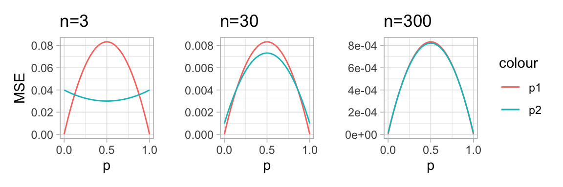
A tale of two estimators

Suppose \(X\sim Binomial(n,p)\) with \(n\) known and \(p\) unknown.

Let \(\hat{p}_1 = X/n\) and let \(\hat{p}_2 = (X+1)/(n+2)\). The effect of the changes in \(\hat{p}_2\) is to nudge the resulting estimate closer to \(0.5\), especially for extreme samples (almost nu successes; almost all successes).

\[ \EE[\hat{p}_1] = \EE\left[X/n\right] = \frac{1}{n}\EE[X] = \frac{1}{n}np = p \]

So the bias of \(\hat{p}_1\) is 0. Hence the MSE is:

\[ MSE_{\hat{p}_1} = \EE[(\hat{p}_1-p)^2] = \VV[\hat{p}_1]+0^2 = \VV\left(\frac{X}{n}\right) = \frac{1}{n^2}\VV[X] = \frac{p(1-p)}{n} \]

A tale of two estimators

Suppose \(X\sim Binomial(n,p)\) with \(n\) known and \(p\) unknown.

Let \(\hat{p}_1 = X/n\) and let \(\hat{p}_2 = (X+1)/(n+2)\).

\[ \EE[\hat{p}_2] = \EE\left[\frac{X+1}{n+2}\right] = \frac{\EE[X]+1}{n+2} = \frac{np+1}{n+2} \]

So the bias is

\[ \EE[\hat{p}_2] - p = \frac{np+1}{n+2}-p = \frac{np+1-p(n+2)}{n+2} = \frac{1-2p}{n+2} = \frac{1/n - 2p/n}{1+2/n} \]

This bias is only 0 when \(p=1/2\). But as \(n\to\infty\), the bias approaches 0. The variance is

\[ \VV[\hat{p}_2] = \VV\left[\frac{X+1}{n+2}\right] = \frac{1}{(n+2)^2}\VV[X] = \frac{np(1-p)}{(n+2)^2} = \frac{p(1-p)}{n+4+4/n} \]

This variance approaches 0 as \(n\to\infty\).

A tale of two estimators

Suppose \(X\sim Binomial(n,p)\) with \(n\) known and \(p\) unknown.

Let \(\hat{p}_1 = X/n\) and let \(\hat{p}_2 = (X+1)/(n+2)\).

As for MSE of \(\hat{p}_2\), we combine the bias and variance terms to get

\[ MSE_{\hat{p}_2} = \VV[\hat{p}_2] + (Bias(\hat{p}_2))^2 = \frac{p(1-p)}{n+4+4/n} + \left(\frac{1/n - 2p/n}{1+2/n}\right)^2 \]

Code

library(tidyverse)
library(patchwork)
library(ggformula)

theme_set(theme_light())
mse.p1 = function(n,p) p*(1-p)/n
mse.p2 = function(n,p) p*(1-p)/(n+4+4/n)+((1/n-2*p/n)/(1+2/n))^2

((
  gf_fun(mse.p1(3,p) ~ p, xlim=c(0,1), color=~"p1", group=~"n=3") %>%
  gf_fun(mse.p2(3,p) ~ p, xlim=c(0,1), color=~"p2", group=~"n=3")
) + scale_x_continuous(breaks=c(0,0.5,1)) + guides(color="none") + xlab("p") + ylab("MSE") + labs(title="n=3")) + ((
  gf_fun(mse.p1(30,p) ~ p, xlim=c(0,1), color=~"p1", group=~"n=30") %>%
  gf_fun(mse.p2(30,p) ~ p, xlim=c(0,1), color=~"p2", group=~"n=30")
) + scale_x_continuous(breaks=c(0,0.5,1)) + guides(color="none") + xlab("p") + ylab("") + labs(title="n=30")) + ((
  gf_fun(mse.p1(300,p) ~ p, xlim=c(0,1), color=~"p1", group=~"n=30") %>%
  gf_fun(mse.p2(300,p) ~ p, xlim=c(0,1), color=~"p2", group=~"n=30")
) + scale_x_continuous(breaks=c(0,0.5,1)) + xlab("p") + ylab("") + labs(title="n=300"))

From the preceding example we learn

Lesson learned

There might not be any universally best estimator.

So maybe we need to restrict our class of estimators. If we choose to study only unbiased estimators, then \(MSE = \VV\), making it easier to optimize.

Definition

A point estimator \(\hat\theta\) of some parameter \(\theta\) is said to be unbiased if \(\EE[\hat\theta]=\theta\).

The bias of an estimator is the difference \(\EE[\hat\theta]-\theta\).

Some unbiased estimators

\(\hat\theta\)	\(\theta\)	Distribution
\(\overline{X}\)	\(\EE[X]\)	all
\(\hat{p}=X/n\)	\(p\)	\(Binomial(p,n)\)

Some biased estimators

\(\hat\theta\)	\(\theta\)	Distribution
\(\max X\)	\(b\)	\(Uniform(a,b)\)
\(\frac{1}{n}\sum(x_i-\mu_X)^2\)	\(\VV\)	all

\(\overline{X}\) is unbiased

Let \(X_1,\dots,X_n\sim\mathcal{D}\) for some distribution \(\mathcal{D}\) with expected value \(\EE[X_i]=\mu\). We compute:

\[ \EE[\overline{X}] = \EE\left[\sum_{i=1}^n X_i/n\right] = \sum_{i=1}^n \EE[X_i]/n = \sum_{i=1}^n \mu/n = n\cdot\mu/n = \mu \]

\(\frac{1}{n}\sum(X_i-\overline{X})^2\) is biased (1/2)

Recall that \(\EE[X^2] = \VV[X] + \EE[X]^2\). We can show \(\frac{1}{n}\sum(X_i-\overline{X})^2 = \frac{1}{n}\sum_i(X_i^2 - \overline{X}^2)\). We compute:

\[ \begin{multline*} \EE\left[\frac{1}{n}\sum_i\left(X_i^2 - \overline{X}^2\right)\right] = \frac{1}{n}\sum_i\EE\left[X_i^2-\overline{X^2}\right] = \frac{1}{n}\sum_i\left(\color{Teal}{\EE\left[X_i^2\right]}-\color{DarkMagenta}{\EE\left[\left(\frac{\sum_j X_j}{n}\right)^2\right]}\right) = \\ \frac{1}{n}\sum_i \left( \color{Teal}{\VV[X_i]+\EE[X_i]^2} - \color{DarkMagenta}{ \left( \VV\left[\frac{\sum_j X_j}{n}\right]+\EE\left[\frac{\sum_j X_j}{n}\right]^2 \right) } \right) = \frac{1}{n}\sum_i\left( \color{Teal}{(\sigma^2+\mu^2)} - \color{DarkMagenta}{\left(n\cdot\frac{\VV[X_j]}{n^2}+\mu^2\right)} \right) \end{multline*} \]

\(\frac{1}{n}\sum(X_i-\overline{X})^2\) is biased (1/2)

The \(\color{Teal}{\mu^2}\) and the \(\color{DarkMagenta}{\mu^2}\) cancel, leaving

\[ \begin{multline*} \EE\left[\frac{1}{n}\sum_i\left(X_i^2 - \overline{X}^2\right)\right] = \frac{1}{n}\sum_i\left( \color{Teal}{\sigma^2} - \color{DarkMagenta}{\left(n\cdot\frac{\VV[X_j]}{n^2}\right)} \right) = \\ \frac{1}{n}\sum_i\left( \sigma^2 - \frac{\sigma^2}{n} \right) = \frac{1}{n}\left(n\sigma^2 - n\frac{\sigma^2}{n}\right) = \sigma^2-\frac{\sigma^2}{n} = \frac{n\sigma^2-\sigma^2}{n} = \frac{n-1}{n}\sigma^2 \end{multline*} \]

Once we see the expected value of the estimator, it is easy to write down an unbiased estimator. Just multiply both sides with \(n/(n-1)\) yielding the usual unbiased estimator \(S^2 = \frac{1}{n-1}\sum(X_i^2-\overline{X}^2)\).

…but unbiased variance ≠ smallest MSE variance

One useful fact about chi-square variables is that \((n-1)S^2/\sigma^2\sim\chi^2(n-1)\). \(\chi^2(n-1)\) has mean \(n-1\) and variance \(2(n-1)\). Write \(X^2 = (n-1)S^2/\sigma^2\).

Consider all estimators \(S_c^2 = c\sum_i(X_i^2-\overline{X}^2)\). Notice that \(S_c^2 = (n-1)S^2c = \sigma^2X^2c\).

Expected value \(\EE[S_c^2]=\EE[\sigma^2X^2c]=\sigma^2\EE[X^2]c=\sigma^2(n-1)c\). Thus the bias is \(\sigma^2(n-1)c-\sigma^2\)

Variance \(\VV[S_c^2]=\VV[\sigma^2X^2c]=\sigma^4c^2\VV[X^2]=\sigma^4\cdot2(n-1)c^2\).

This yields \[ \begin{multline*} MSE = \VV+Bias^2 = \sigma^4\cdot2(n-1)c^2 + (\sigma^2(n-1)c - \sigma^2)^2 = \\ 2(n-1)\sigma^4c^2 + (n-1)^2\sigma^4c^2-2(n-1)\sigma^2c + \sigma^4 = \\ c^2\sigma^4(2(n-1)+(n-1)^2) + c\sigma^4(-2(n-1)) + \sigma^4 \end{multline*} \]

…but unbiased variance ≠ smallest MSE variance

To minimize MSE, take \(dMSE/dc\) and solve for \(c\):

\[ \begin{multline*} \frac{dMSE}{dc} = 2c\sigma^4(2(n-1)+(n-1)^2) + \sigma^4(-2(n-1))\\ \text{which is 0 when } c=\frac{\color{Teal}{\sigma^4}\cdot\color{DarkMagenta}{2}(n-1)}{\color{DarkMagenta}{2}\cdot\color{Teal}{\sigma^4}(\color{GoldenRod}{2n}\color{Crimson}{-2}+n^2\color{GoldenRod}{-2n}+\color{Crimson}{1})} = \frac{n-1}{n^2\color{Crimson}{-1}} = \frac{1}{n+1} \end{multline*} \]

So the only unbiased estimator is with \(c=1/(n-1)\) and the estimator with minimal MSE is with \(c=1/(n+1)\).

…and unbiased variance does not yield unbiased standard deviation

Definition

A function \(f\) is convex (concave) if for any \(x,y\), the chord connecting \((x,f(x))\) to \((y,f(y))\) lies above (below) the graph of \(f\).

One important theorem is

Theorem (Jensen’s Inequality)

If \(f\) is convex (concave), then

\[ f(\EE[X]) \leq \EE[f(X)] \qquad (\quad f(\EE[X]) \geq \EE[f(X)]\quad) \]

with strict inequality unless \(f\) is linear.

Since \(\sqrt\) is concave, \(\EE[\sqrt{S^2}] < \sigma\) and thus \(\sqrt{S^2}\) is a biased estimator of the standard deviation.

Minimum Variance Unbiased Estimators (MVUE)

Let’s soldier on and focus on unbiased estimators. Among these, the bias term in \(MSE\) vanishes, and so a minimum MSE unbiased estimator is one with minimum variance.

Example: the continuous German Tank Problem

Suppose \(X_1,\dots,X_n\sim Uniform(0,\theta)\). Our challenge is to estimate the value of \(\theta\) based on observations of the \(X_i\).

Idea: use the mean

The expected value of a \(X\sim Uniform(0,\theta)\) is

\[ \begin{multline*} \EE[X] = \int_0^\theta x \cdot \frac{1}{\theta} dx = \\ \frac{1}{\theta}\left[\frac{x^2}{2}\right]_0^\theta = \frac{1}{\theta}\left(\frac{\theta^2}{2}-\frac{0}{2}\right) = \frac{\theta}{2} \end{multline*} \]

So maybe \(2\overline{X}\) might work?

(this is an instance of the Method of Moments that we will meet later)

Idea: use the max

If we actually observe some value \(x\), then certainly \(\theta\geq x\), because the probability density is 0 outside the support.

So maybe \(\max\{X_i\}\) could work?

Aside: Order Statistics

To understand the max, we need a bit more theory to get it right - we need to know about order statistics.

Given \(X_1,\dots,X_n\sim\mathcal{D}\), write \(X_{(j)}\) for the \(j\)th biggest value among the \(X_i\), so that \(X_{(1)}\leq X_{(2)}\leq\dots\leq X_{(n)}\).

We will derive the PDF for \(X_{(j)}\) based on the PDF and CDF of \(\mathcal{D}\) (assuming that \(\mathcal{D}\) is a continuous distribution)

Let \(\delta x\) be a small value, so that the interval \((x, x+\delta x]\) is small enough for it to be unlikely to contain two of the \(X_i\). We split \(\RR\) into three components:

• \(\color{Teal}{(-\infty, x]}\) with \(\PP = CDF(x)\)
• \(\color{DarkMagenta}{(x, x+\delta x]}\) with \(\PP \approx PDF(x)\cdot\delta x\)
• \(\color{GoldenRod}{(x+\delta x, \infty)}\) with \(\PP = 1-CDF(x+\delta x)\)

The middle interval contains \(X_{(j)}\) precisely if the first interval contains \(j-1\) of the \(X_i\), the middle interval contains exactly \(1\) of the \(X_i\), and the last interval contains \(n-j\) of the \(X_i\).

Aside: Order Statistics

This setup - three classes, prescribed # of elements falling in each, fixed probabilities for each class - is exactly the setup for the multinomial distribution (ch. 5.1). So we can write down the probability

\[ \begin{multline*} CDF(x+\delta x)-CDF(x) = \PP(x < X_{(j)} \leq x+\delta x) \approx \\ \frac{n!}{(j-1)!\,\,1!\,\,(n-j)!} \color{Teal}{CDF(x)^{j-1}}\cdot \color{DarkMagenta}{PDF(x)\cdot\delta x }\cdot \color{GoldenRod}{(1-CDF(x+\delta x))^{n-j}} \end{multline*} \]

Divide by \(\delta x\) and take the limit as \(\delta x\to0\) and we get (by the definition of the derivative)

\[ PDF_{X_{(j)}}(x) = \frac{n!}{(j-1)!\,\,1!\,\,(n-j)!} {CDF(x)^{j-1}}\cdot {PDF(x) }\cdot {(1-CDF(x+\delta x))^{n-j}} \]

In particular:

• \(PDF_{\min X_i}(x) = n\cdot PDF(x)\cdot(1-CDF(x))^{n-1}\)
• \(PDF_{\max X_i}(x) = n\cdot PDF(x)\cdot CDF(x)^{n-1}\)

MVUE - Continuous German Tank

The sample mean is unbiased (in general) for the population mean, so \(2\overline{X}\) is unbiased.

For the max, we can compute

\[ \begin{multline*} \EE[X_{(n)}] = \int_0^\theta x \cdot PDF_{X_{(j)}}(x)dx = \\ \int_0^\theta x \cdot n\cdot PDF(x) \cdot CDF(x)^{n-1}dx = \\ \int_0^\theta x \cdot n\cdot \frac{1}{\theta} \cdot \frac{x^{n-1}}{\theta^{n-1}} dx = \int_0^\theta n\frac{x^n}{\theta^n}dx = \frac{n}{n+1}\theta \end{multline*} \]

So \(\max\{X_i\}\) is not unbiased - however, \(\frac{n+1}{n}\theta\) is.

MVUE - Continuous German Tank

Since both \(2\overline{X}\) and \(\frac{n+1}{n} X_{(n)}\) are unbiased, we only need to compare their variances. We know (or can look up) that the variance of \(Uniform(0,\theta)\) is \(\theta^2/12\).

\[ \VV[2\overline{X}] = 4\VV[\overline{X}] = 4n\frac{\VV[X_i]}{n^2} = 4\frac{\theta^2/12}{n} = \frac{\theta^2}{3n} \]

Using maximum likelihood estimation (exercise 7.50, homework in 2 weeks) we can derive

\[ \VV\left[\frac{n+1}{n}X_{(n)}\right] = \frac{\theta^2}{n(n+2)} \]

For \(n>2\), we get that the bias-adjusted maximum has lower variance - and it can be shown that this is true for all other possible unbiased estimators.

Precision for estimators: Standard Error

Definition

The standard error of an estimator \(\hat\theta\) is its standard deviation \(\sigma_{\hat\theta} = \sqrt{\VV[\hat\theta]}\).

If this standard error requires estimated quantities, using estimates yields the estimated standard error \(s_{\hat\theta}\) or \(\hat\sigma_{\hat\theta}\).

Example: standard error of sample proportion

(Exercise 7.2) A sample of 20 students turned out to have owned Texas Instruments (T), Hewlett-Packard (H), Casio (C) or Sharp (S) calculators:

T T H T C T T S C H S S T H C T T T H T

Estimate \(\PP(\text{student owns TI})\).

T: 10, H: 4, C: 3, S: 3

We calculate \(\hat{p} = \#T/n = 10/20 = 1/2\).

We know that the binomial distribution has \(\VV=pq/n\), so \(s_{\hat{p}} = \sqrt{\hat\VV} = \sqrt{(1/2\cdot 1/2) / n} = \sqrt{1/80} \approx 0.1118 = 11.18\%u\).

Bootstrap estimation of standard errors

You might have an estimator that is difficult or complicated to analyze. Computers can help, using the bootstrap method.

Basic idea

1. Treat the sample you have as an empiric random distribution.
2. Draw new samples at random from the empiric distribution.
3. Study whatever you need to know about the sample distribution from these new samples.

Bootstrap example

(R, using tidyverse and foreach)

Continue the Exercise 7.2 example:

Code

library(tidyverse)
library(foreach)
B=1000
calculators = tibble(
  c=factor(c('T','T','H','T','C','T','T','S','C','H',
             'S','S','T','H','C','T','T','T','H','T')) )
boot.prop = foreach(1:1000, .combine=rbind) %do% 
  ( calculators %>% slice_sample(prop=1.0, replace=TRUE) %>%
    summarise(p.hat=mean(c=='T')) )
c(p.hat = mean(boot.prop$p.hat), std.err = sd(boot.prop$p.hat))

    p.hat   std.err 
0.5049500 0.1146348 

Compare with our previous analytic result of \(\hat{p}=0.5\) and \(s_{\hat{p}} \approx 0.1118\).

Bootstrap example

(R, using boot)

Continue the Exercise 7.2 example:

Code

library(tidyverse)
library(boot)
B=1000
calculators = tibble(
  c=factor(c('T','T','H','T','C','T','T','S','C','H',
             'S','S','T','H','C','T','T','T','H','T')) )
prop.TI = function(data,weights) mean(data$c[weights] == 'T')
boot.prop = boot(calculators, prop.TI, B)
boot.prop

ORDINARY NONPARAMETRIC BOOTSTRAP


Call:
boot(data = calculators, statistic = prop.TI, R = B)


Bootstrap Statistics :
    original   bias    std. error
t1*      0.5 -0.00195   0.1137173

Compare with our previous analytic result of \(\hat{p}=0.5\) and \(s_{\hat{p}} \approx 0.1118\).

Good platforms for writing up your homework

Both these platforms can compile to PDF which you then can upload to Blackboard for your homework solutions.

LaTeX

• Standard markup language for writing mathematical text
• Standard markup language for writing mathematical formulas
• Easy access (no software installation for yourself) through https://overleaf.com
• https://en.wikibooks.org/wiki/LaTeX is a very good introduction and reference
• This is how I write all my papers

Quarto (…or RMarkdown)

• Uses Markdown as a formatting markup language
• Integrates running code (in R, Python, Julia, and more) directly into the document itself
• This is how I write these slides