Lecture 5: Geometric Representation

Today’s Visualization

Marks and Channels

Marks in data visualization

A mark is a basic graphical element in an image.

Munzner shows examples of points, lines, curves, areas.

Wilkinson’s taxonomy of marks is bigger

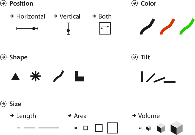
Channels - the appearance of marks

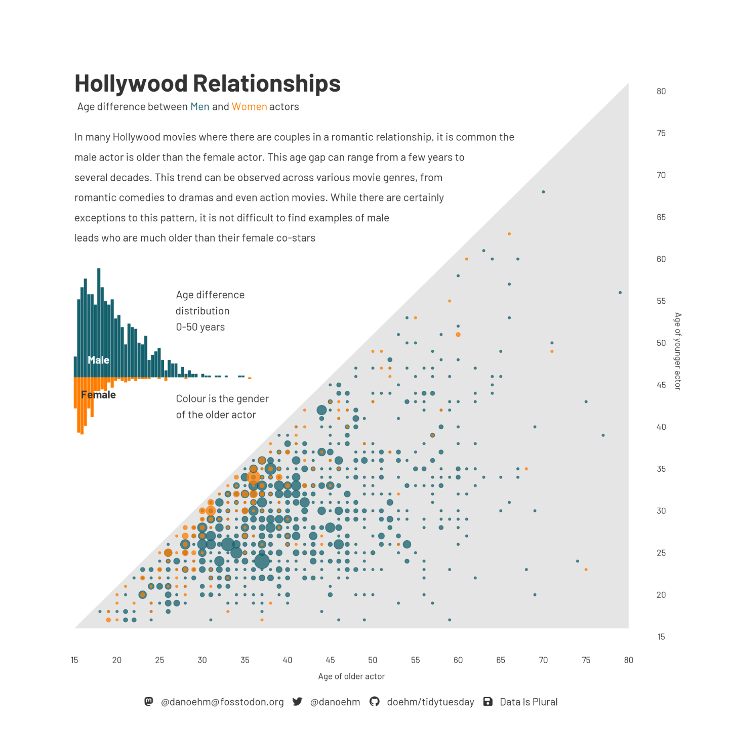
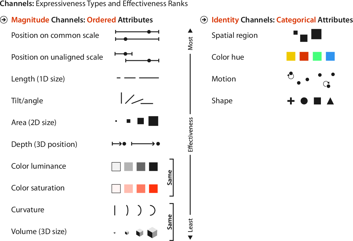
Visual channels are different ways of controlling the appearance of marks. The core of data visualization design lies in the connection between visual channels and data properties.

Design Principles for Visual Channels

Expressiveness

Visual encoding should express all of, and only, the information in the dataset attributes. Ordered data should be shown in a way that our perceptual system intrinsically senses as ordered. Conversely, unordered data should not be shown in a way that perceptually implies an ordering that does not exist.

Effectiveness

The importance of the attribute should match the salience of the channel. The most important attributes should be encoded with the most effective channels in order to be most noticeable, and then decreasingly important attributes can be matched with less effective channels.

Visual channels in use

Code

fig = pyplot.figure()
ax = fig.subplots()

styles = [
  matplotlib.markers.MarkerStyle("d"),
  matplotlib.markers.MarkerStyle("s")
]
colors = ["blue", "blue"]
faces = ["blue", "blue"]
for (x,y),c in zip(data.T, cat):
  _ = ax.plot(x, y, marker=styles[c], 
          markeredgecolor=colors[c], 
          markerfacecolor=faces[c])

_ = pyplot.axis("square")
pyplot.show()

Categorical: Shape

Visual channels in use

Code

fig = pyplot.figure()
ax = fig.subplots()

styles = [
  matplotlib.markers.MarkerStyle("|"),
  matplotlib.markers.MarkerStyle("|", 
    transform=matplotlib.transforms.Affine2D().rotate_deg(-30))
]
colors = ["blue", "blue"]
faces = ["blue", "blue"]
for (x,y),c in zip(data.T, cat):
  _ = ax.plot(x, y, marker=styles[c], 
          markeredgecolor=colors[c], 
          markerfacecolor=faces[c])

_ = pyplot.axis("square")
pyplot.show()

Categorical: Tilt

Visual channels in use

Code

fig = pyplot.figure()
ax = fig.subplots()

styles = [
  matplotlib.markers.MarkerStyle("|"),
  matplotlib.markers.MarkerStyle("|", 
    transform=matplotlib.transforms.Affine2D().scale(1.5))
]
colors = ["blue", "blue"]
faces = ["blue", "blue"]
for (x,y),c in zip(data.T, cat):
  _ = ax.plot(x, y, marker=styles[c], 
          markeredgecolor=colors[c], 
          markerfacecolor=faces[c])

_ = pyplot.axis("square")
pyplot.show()

Categorical: Size

Visual channels in use

Code

fig = pyplot.figure()
ax = fig.subplots()

styles = [
  matplotlib.markers.MarkerStyle("|"),
  matplotlib.markers.MarkerStyle("|")
]
colors = ["blue", "red"]
faces = ["blue", "red"]
for (x,y),c in zip(data.T, cat):
  _ = ax.plot(x, y, marker=styles[c], 
          markeredgecolor=colors[c], 
          markerfacecolor=faces[c])

_ = pyplot.axis("square")
pyplot.show()

Categorical: Color

Visual channels in use

Code

fig = pyplot.figure()
ax = fig.subplots()

styles = [
  matplotlib.markers.MarkerStyle("|", 
    transform=matplotlib.transforms.Affine2D().rotate_deg(-15*i)) for i in range(bins.min(),bins.max()+1)
]
colors = ["blue"]*10
faces = ["blue"]*10
for (x,y),o in zip(data.T, bins):
  _ = ax.plot(x, y, marker=styles[o-1], 
          markeredgecolor=colors[o-1], 
          markerfacecolor=faces[o-1])

_ = pyplot.axis("square")
pyplot.show()

Ordinal: Tilt

Visual channels in use

Code

fig = pyplot.figure()
ax = fig.subplots()

styles = [
  matplotlib.markers.MarkerStyle("2", 
    transform=matplotlib.transforms.Affine2D().scale(1.2**i)) for i in range(bins.min(),bins.max()+1)
]
colors = ["blue"]*10
faces = ["blue"]*10
for (x,y),o in zip(data.T, bins):
  _ = ax.plot(x, y, marker=styles[o-1], 
          markeredgecolor=colors[o-1], 
          markerfacecolor=faces[o-1])

_ = pyplot.axis("square")
pyplot.show()

Ordinal: Area

Visual channels in use

Code

fig = pyplot.figure()
ax = fig.subplots()

styles = [matplotlib.markers.MarkerStyle("2")]*5
colors = [f"#6495ED{x:02x}" for x in np.linspace(0, 256, 6, dtype="uint8")[1:]]
faces = colors
for (x,y),o in zip(data.T, bins):
  _ = ax.plot(x, y, marker=styles[o-1], 
          markeredgecolor=colors[o-1], 
          markerfacecolor=faces[o-1])

_ = pyplot.axis("square")
pyplot.show()

Ordinal: Transparency

Visual channels in use

Code

fig = pyplot.figure()
ax = fig.subplots()
r,g,b = matplotlib.colors.to_rgb("#6495ed")
h,s,v = matplotlib.colors.rgb_to_hsv([r,g,b])
styles = [matplotlib.markers.MarkerStyle("2")]*5
colors = [matplotlib.colors.hsv_to_rgb((h,s,vv)) for vv in np.linspace(0,1,6)[1:]]
faces = colors
for (x,y),o in zip(data.T, bins):
  _ = ax.plot(x, y, marker=styles[o-1], 
          markeredgecolor=colors[o-1], 
          markerfacecolor=faces[o-1])

_ = pyplot.axis("square")
pyplot.show()

Ordinal: Luminance

Visual channels in use

Code

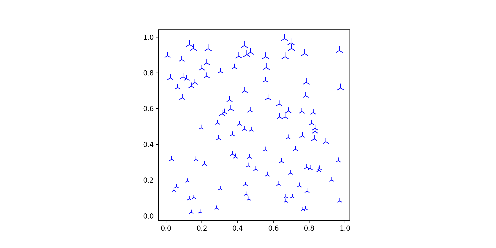
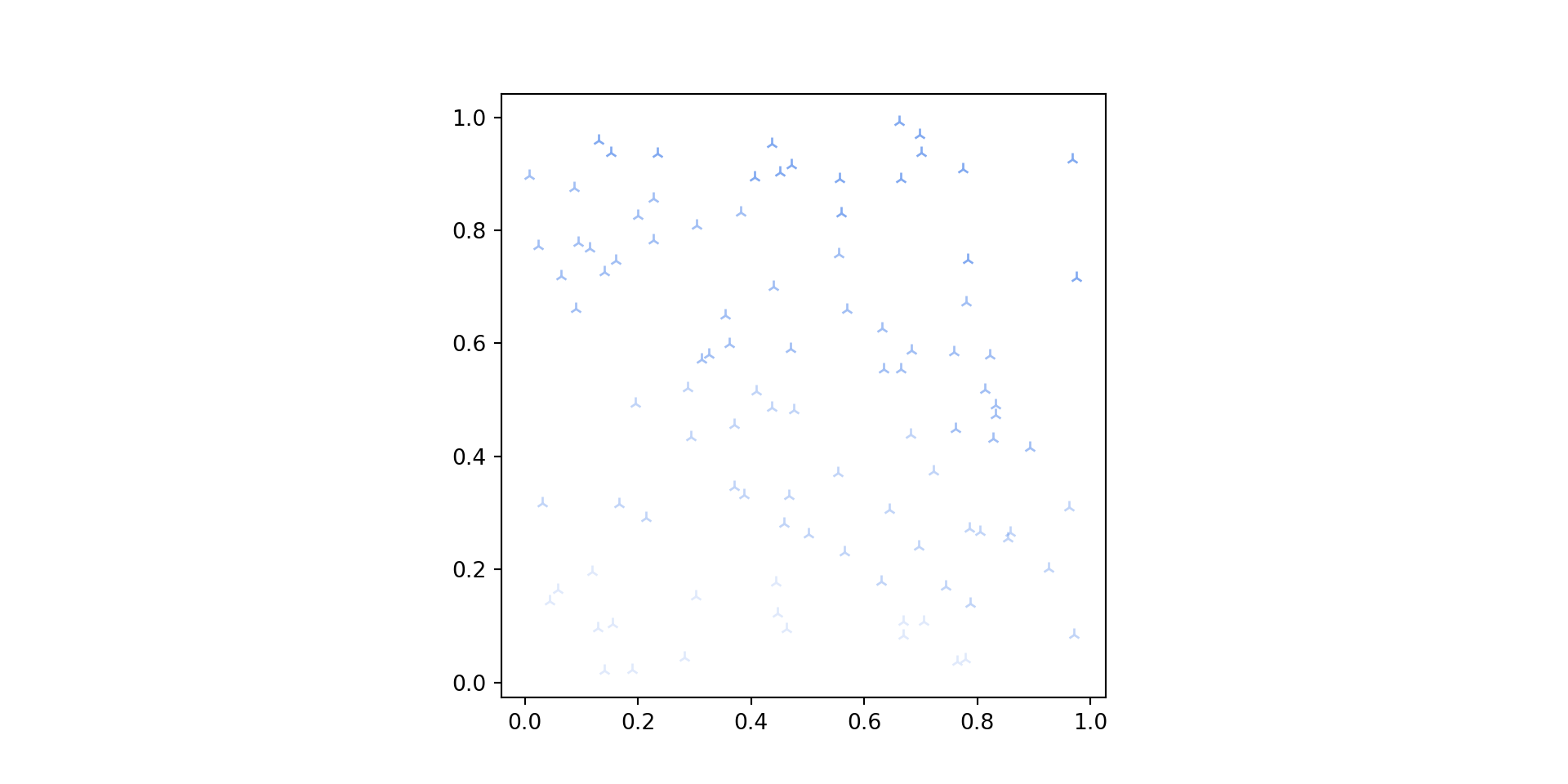
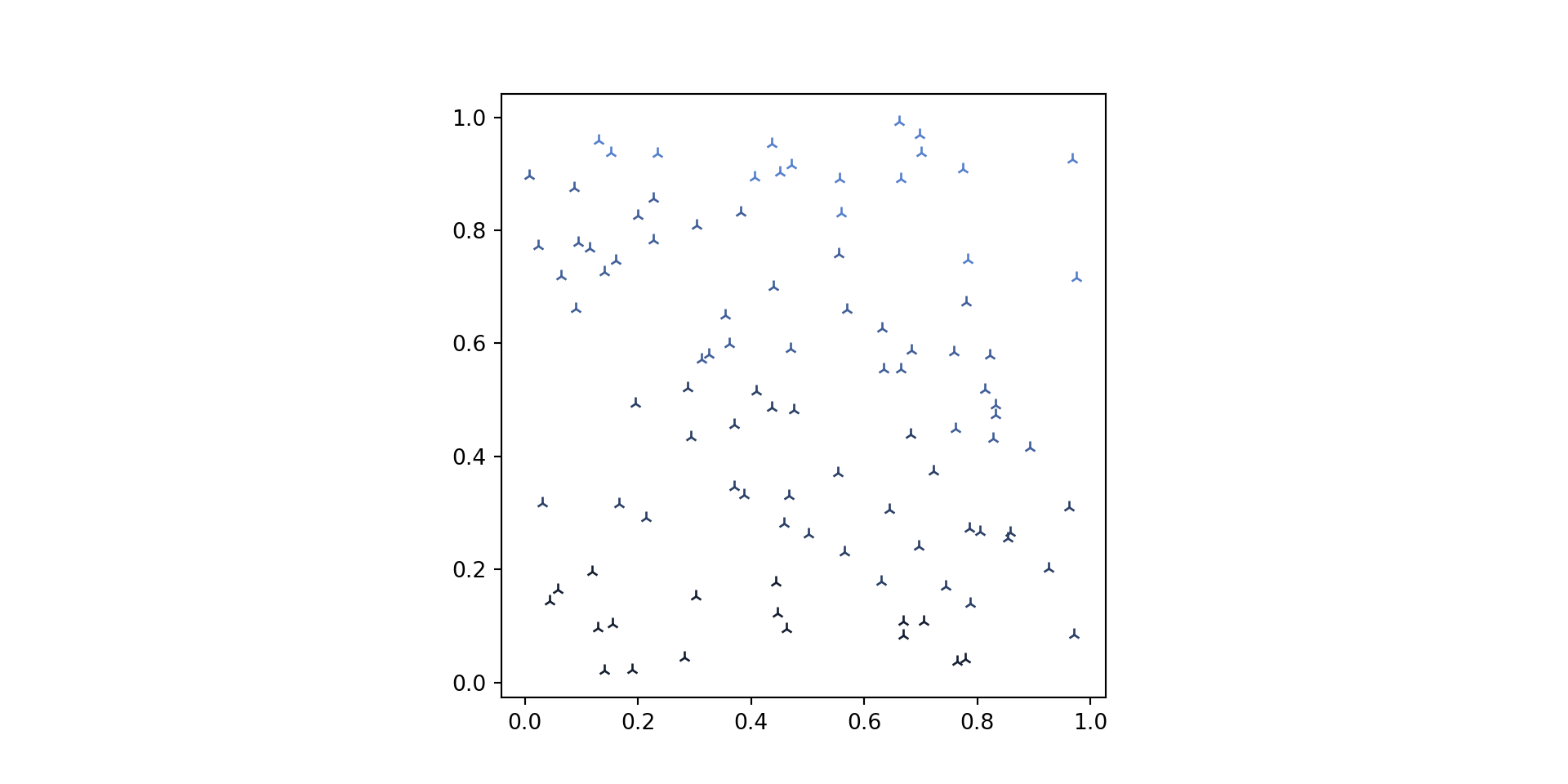
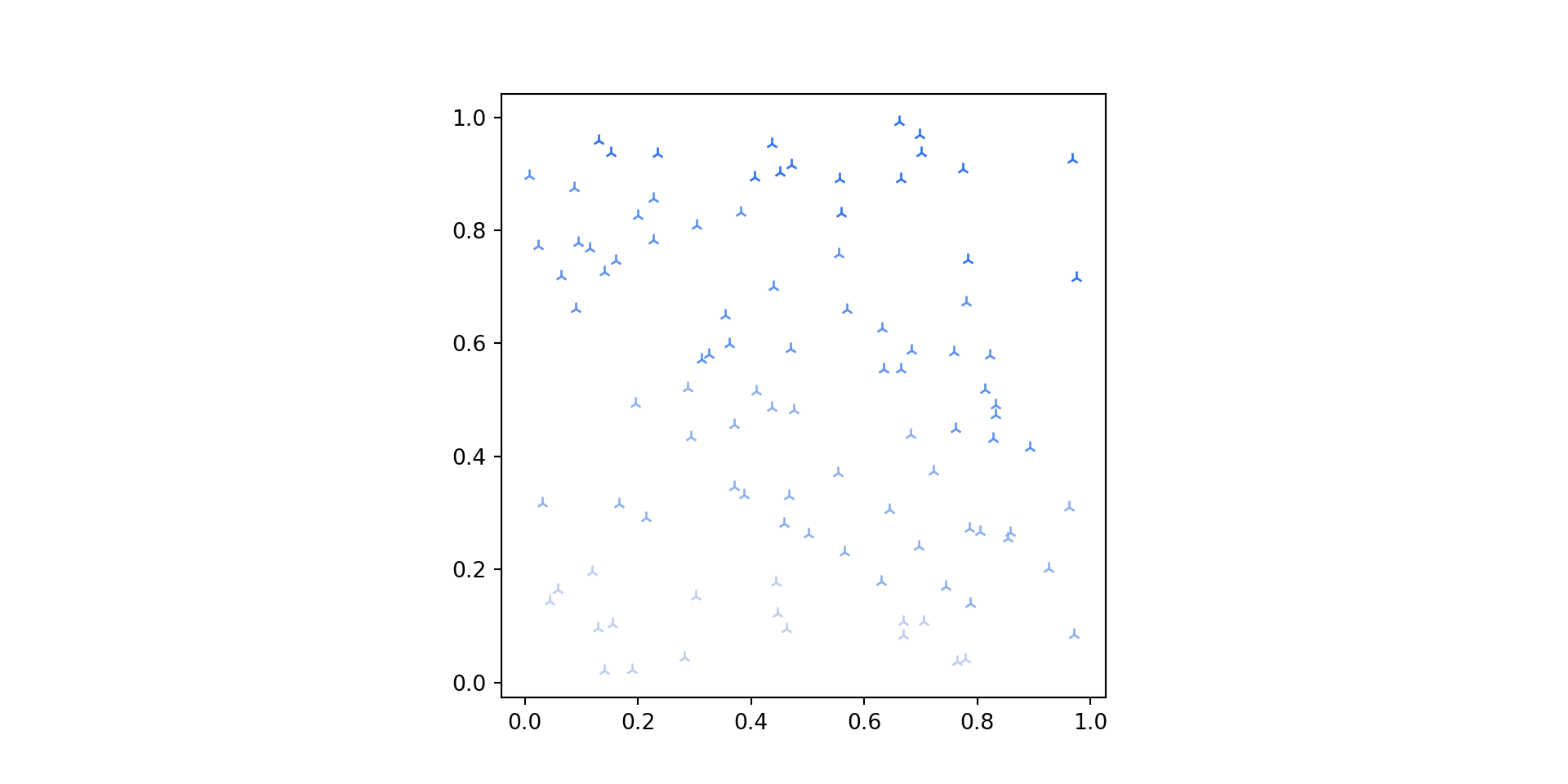
fig = pyplot.figure()
ax = fig.subplots()
r,g,b = matplotlib.colors.to_rgb("#6495ed")
h,s,v = matplotlib.colors.rgb_to_hsv([r,g,b])
styles = [matplotlib.markers.MarkerStyle("2")]*5
colors = [matplotlib.colors.hsv_to_rgb((h,ss,v)) for ss in np.linspace(0,1,6)[1:]]
faces = colors
for (x,y),o in zip(data.T, bins):
  _ = ax.plot(x, y, marker=styles[o-1], 
          markeredgecolor=colors[o-1], 
          markerfacecolor=faces[o-1])

_ = pyplot.axis("square")
pyplot.show()

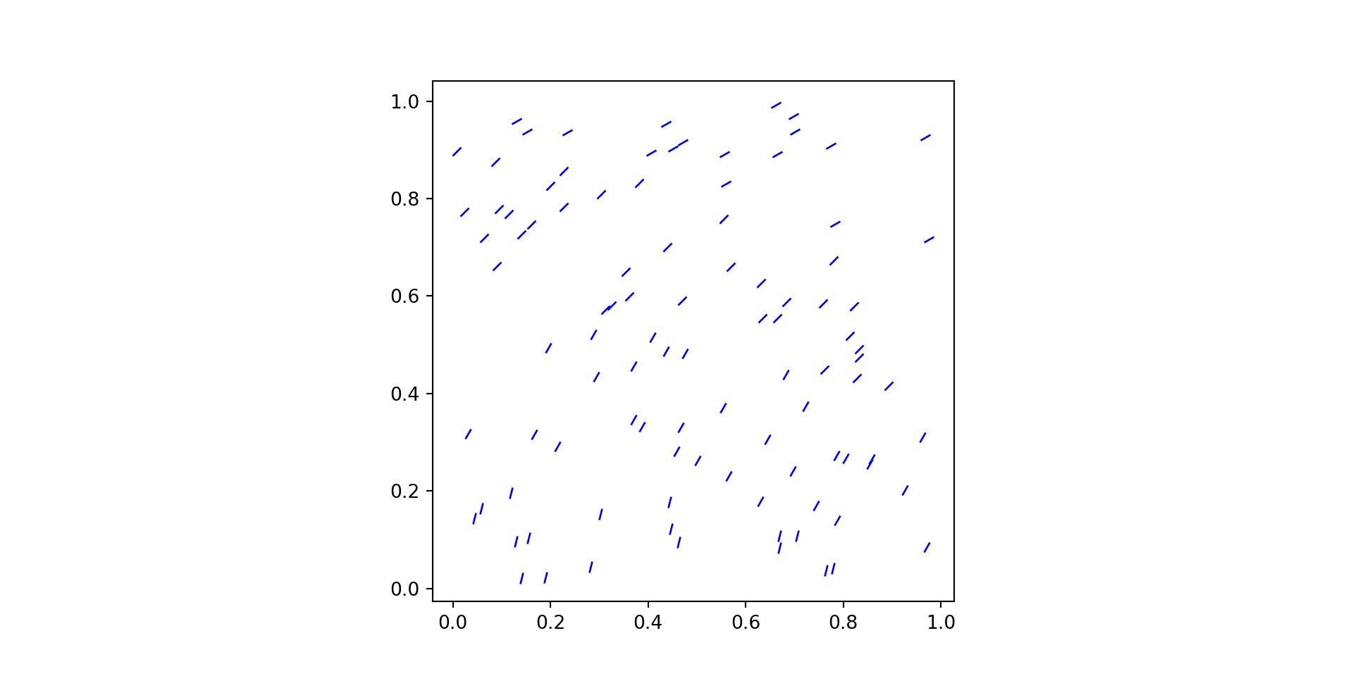
Ordinal: Saturation

Channel Efficiency: experiments

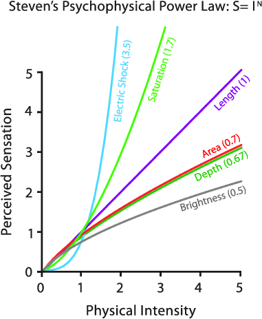
Stevens (1975): human response to sensory stimulus is characterized by a power law, with different exponents for different stimulus modality. Asked ratio judgements and fitted power law curves.

Continuum	Exponent ()	Stimulus condition
Loudness	0.67	Sound pressure of 3000 Hz tone
Vibration	0.95	Amplitude of 60 Hz on finger
Vibration	0.60	Amplitude of 250 Hz on finger
Brightness	0.33	5° target in dark
Brightness	0.50	Point source
Brightness	0.50	Brief flash
Brightness	1.00	Point source briefly flashed
Lightness	1.20	Reflectance of gray papers
Visual length	1.00	Projected line
Visual area	0.70	Projected square
Redness (saturation)	1.70	Red–gray mixture
Taste	1.30	Sucrose
Taste	1.40	Salt
Taste	0.80	Saccharin
Smell	0.60	Heptane
Cold	1.00	Metal contact on arm
Warmth	1.60	Metal contact on arm
Warmth	1.30	Irradiation of skin, small area
Warmth	0.70	Irradiation of skin, large area
Discomfort, cold	1.70	Whole-body irradiation
Discomfort, warm	0.70	Whole-body irradiation
Thermal pain	1.00	Radiant heat on skin
Tactual roughness	1.50	Rubbing emery cloths
Tactual hardness	0.80	Squeezing rubber
Finger span	1.30	Thickness of blocks
Pressure on palm	1.10	Static force on skin
Muscle force	1.70	Static contractions
Heaviness	1.45	Lifted weights
Viscosity	0.42	Stirring silicone fluids
Electric shock	3.50	Current through fingers
Vocal effort	1.10	Vocal sound pressure
Angular acceleration	1.40	5 s rotation
Duration	1.10	White-noise stimuli

Channel Efficiency: experiments

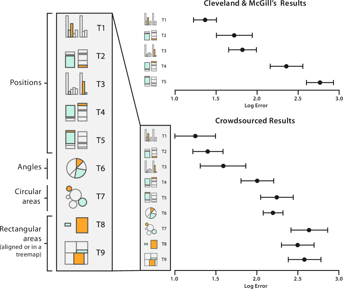
Cleveland and McGill (1984) and Heer and Bostock (2010): controlled experiments ranking perceptual accuracy in reading visualizations.

Perceptual ranking of channels

Measures of efficiency

Accuracy

The preceding examples all focus on accuracy.

Discriminability

Are the intended differences perceptible to the human? How many bins can be used in a particular channel?

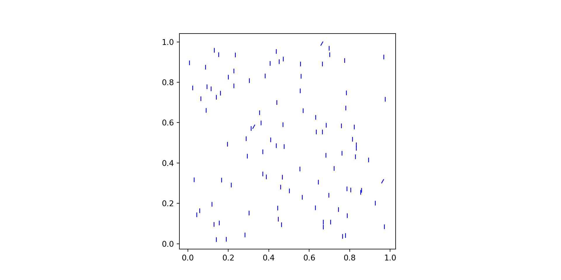
Separability

Different channels interact with each other.

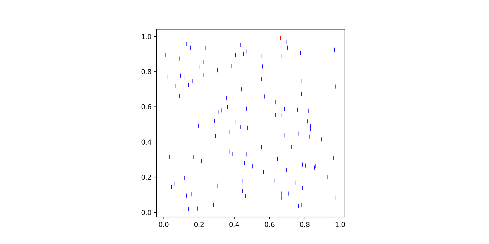
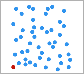
Popout

How much does a distinct item stand out from many other items? This leverages the parallel processing in the low-level visual system.

Discriminability

Separability

Visual channels are:

separable if they are orthogonal and independent.
integral if they are inextricably combined.

If you try to encode different information in integral channels, the encoding will fail. Instead of accessing the desired information about each attribute, an unanticipated combination is perceived.

Example: vertical position, horizontal position and proximity. Once you have two of these, you cannot encode an independent attribute in the third.

Example: red, green, blue color channels have a lot of integration.

Separability

Popout

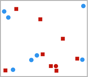
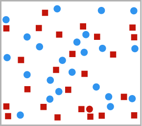
Detection time for the red circle approximately constant wrt # distractors.

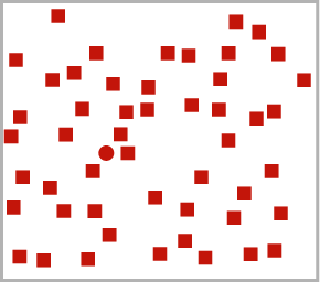
Popout

Detection time for the red circle approximately linear wrt # distractors. Square vs circle yields less popout than blue vs red.

Popout

Detection time for the red circle approximately linear wrt # distractors. A mix of visual channels does not preserve popout properties.

Minard’s March on Moscow

Work in pairs. Carefully describe all aspects of this graphic. What do you notice?

Minard’s March on Moscow

Some things MVJ notices:

Time is represented by east-west position
Temperature line graph at the bottom synched with return march progress.
Very sparse geography representation to help a reader orient.
Chart-crossing lines to guide the reader associating temperature chart to army positions.

Minard’s March on Moscow

Homework: Recreate Minard’s March on Moscow chart as faithfully as you can on your chosen platform. Blackboard has data files with positions of the cities, extents of the paths, and data for the temperature chart.

If you want the rivers, you may have to find corresponding data yourself.