---

Another example using R

Load the packages:

library(TDA)
library(deldir)

Generate some sample data sets:

Y <- {
  theta <- runif(200, 0, 2*pi)
  radius <- c( runif(100, 0.4, 0.5), runif(100, 1, 1.1) )
  x <- radius * cos(theta)
  y <- radius * sin(theta)
  cbind(x, y)
}

Plot it:

plot(Y, pch=20, col='blue', asp=1)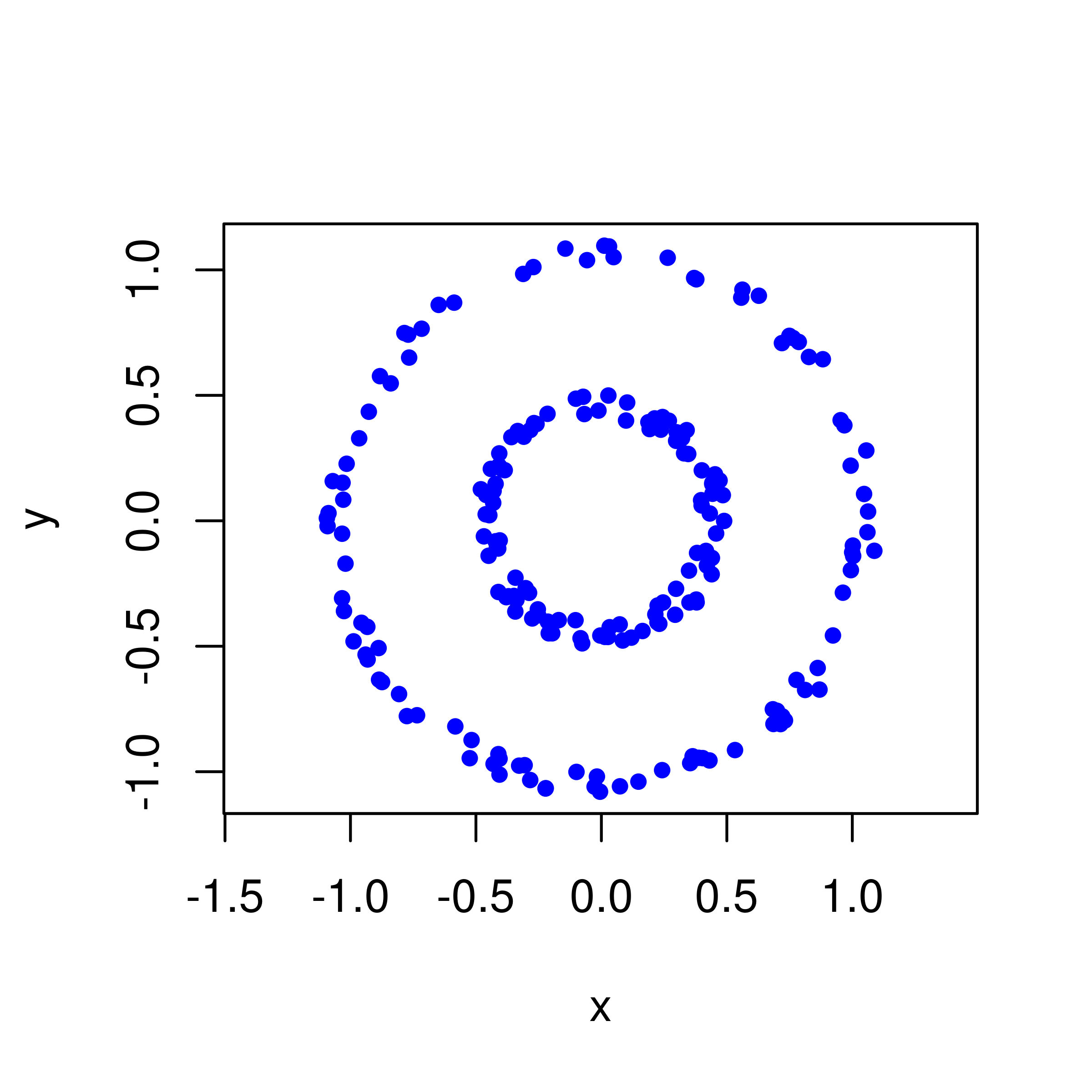

Now look at the persistence diagram:

PH.output <- alphaComplexDiag(Y)
PD <- PH.output[["diagram"]]
plot(PD, asp=1, diagLim = c(0,0.3))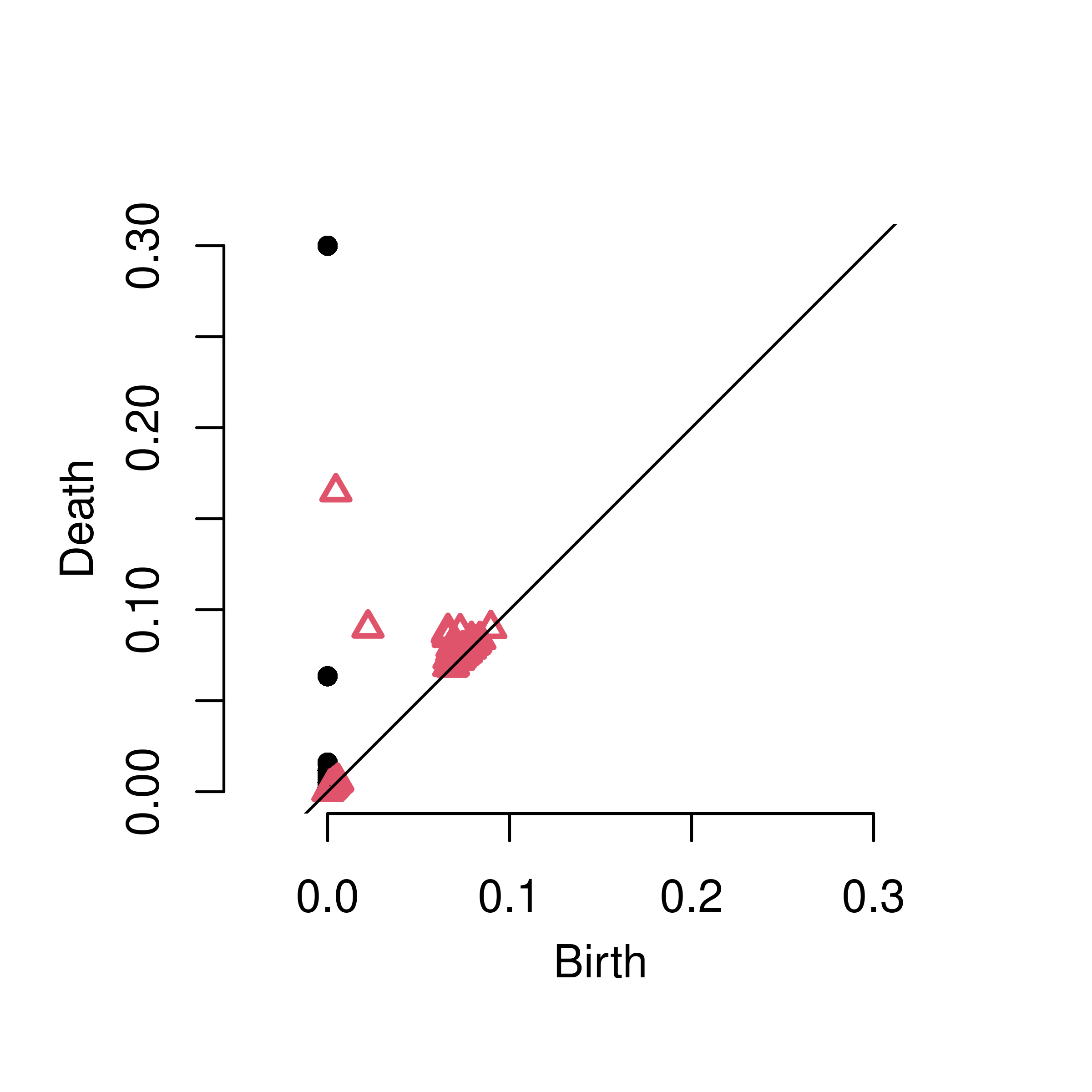

Here’s the barcode:

plot(PD, diagLim = c(0,0.3), barcode=TRUE)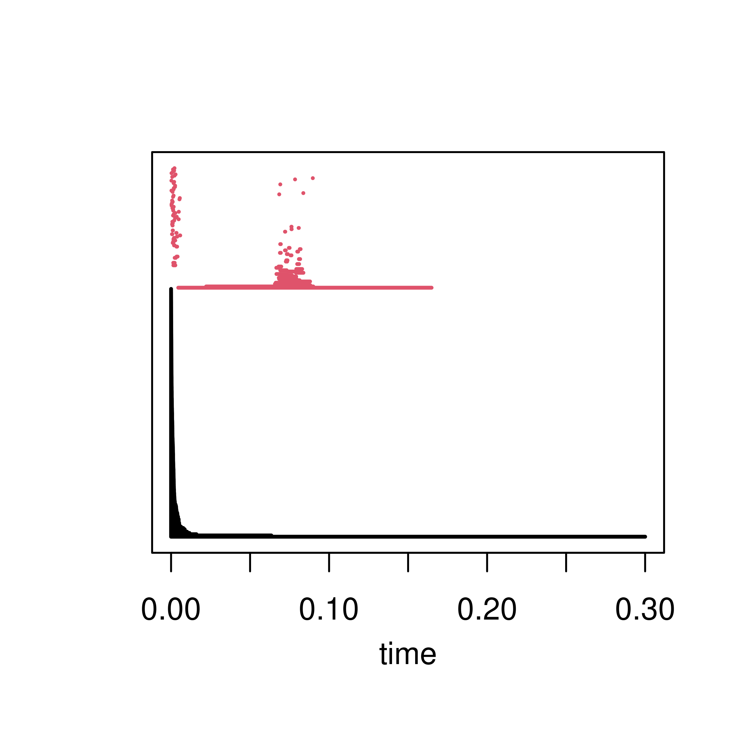

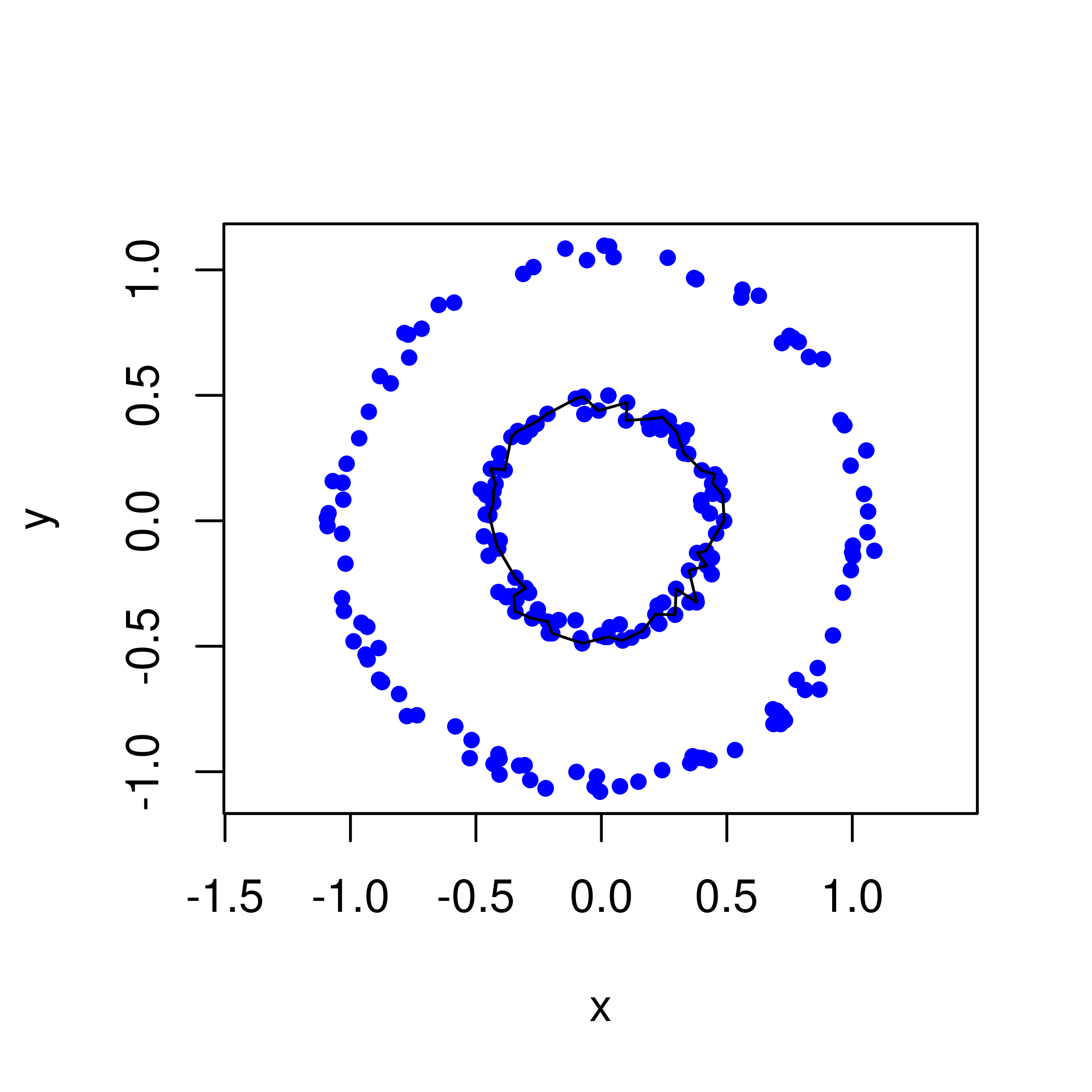
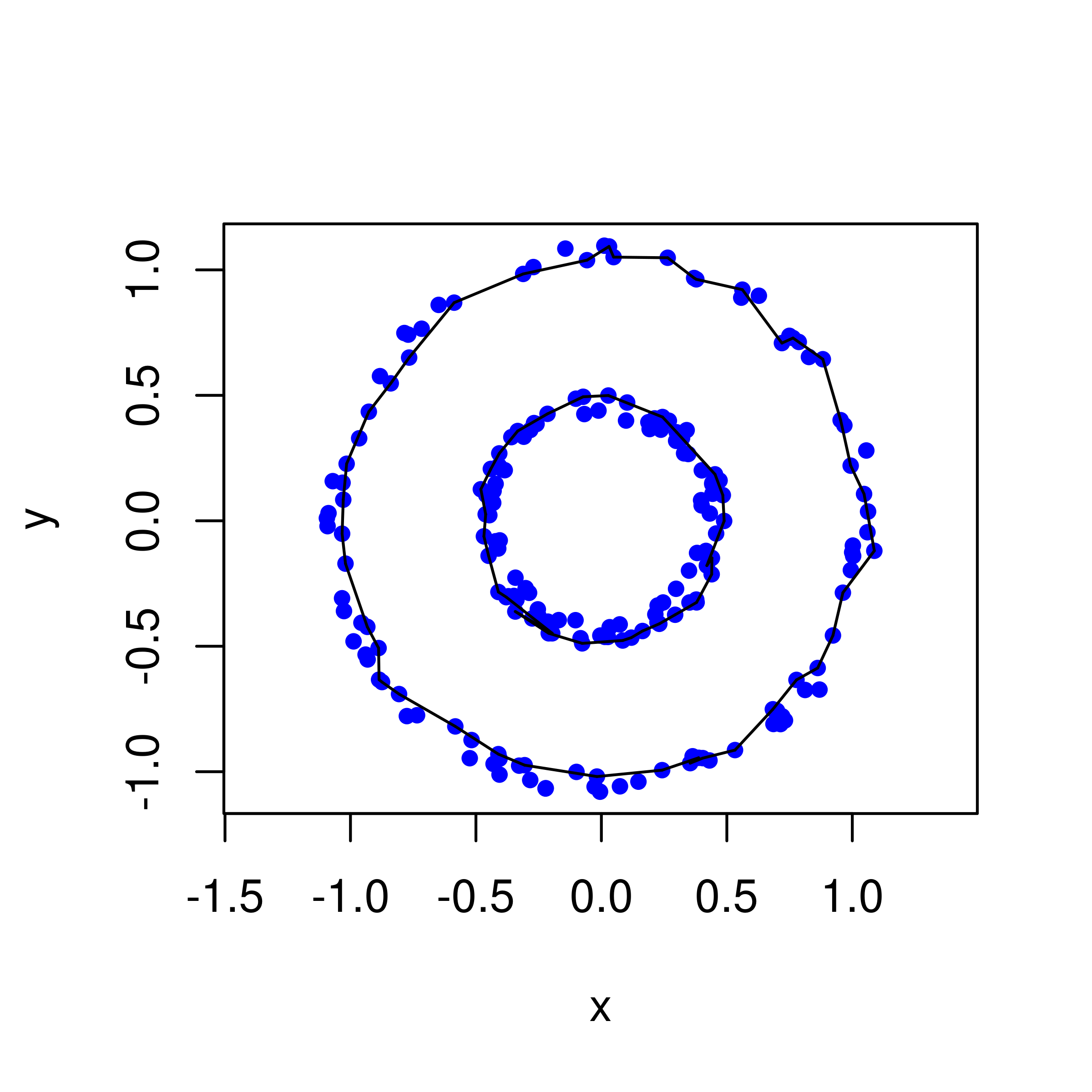
Now plot the two longest persistent cycles.

PH.output <- ripsDiag(Y, maxdimension = 1, maxscale = max.filtration, library = c("GUDHI", "Dionysus"), location = TRUE)
PD <- PH.output[["diagram"]]
ones <- which(PD[, 1] == 1)
persistence <- PD[ones,3] - PD[ones,2]
cycles <- PH.output[["cycleLocation"]][ones[order(persistence, decreasing=TRUE)]]
plot(Y, pch=20, col='blue', asp=1)
for (i in 1:dim(cycles[[1]])[1]){
    lines(cycles[[1]][i,,])
}
plot(Y, pch=20, col='blue', asp=1)
for (i in 1:dim(cycles[[2]])[1]){
    lines(cycles[[2]][i,,])
}

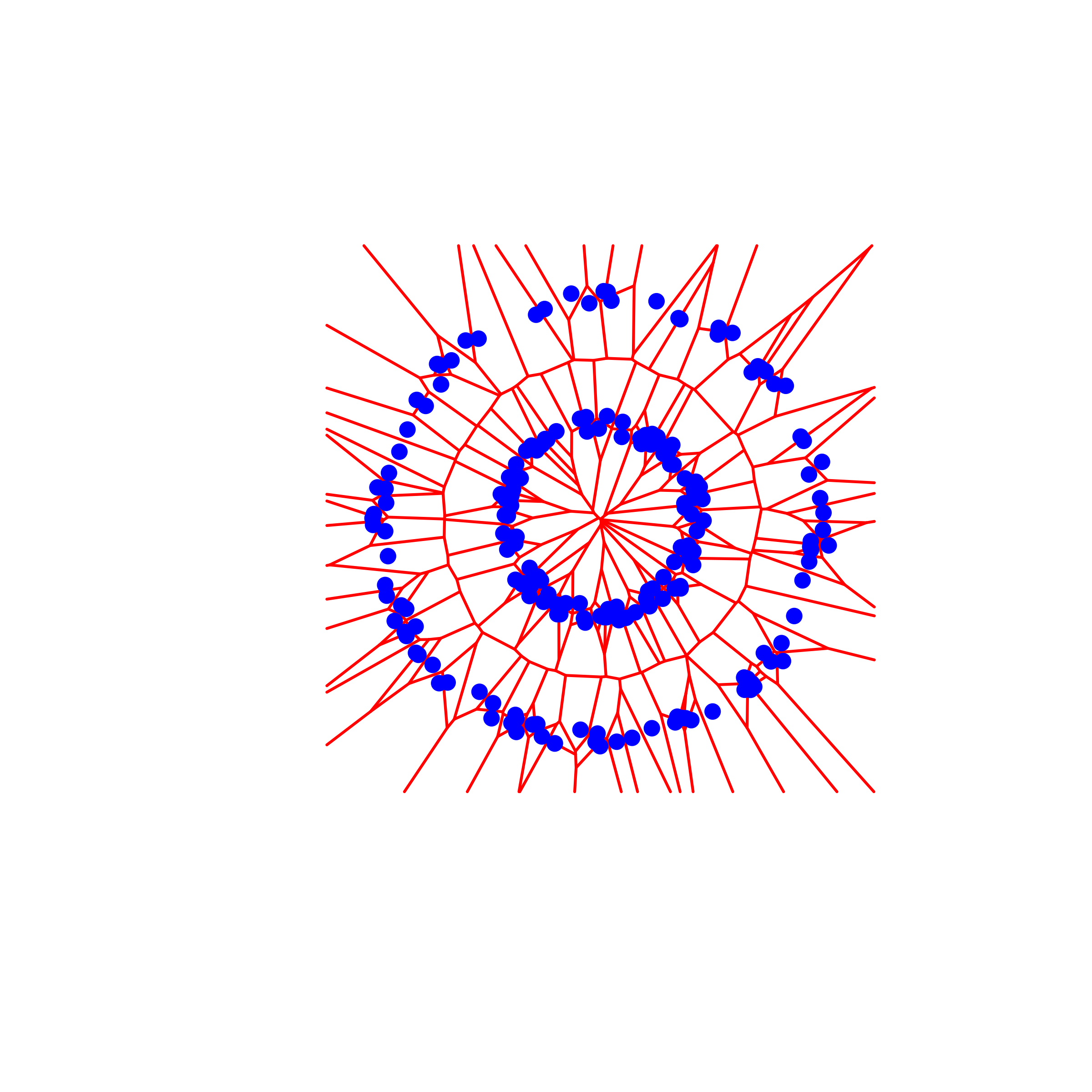
We can read off the correct scale for the clusters from the persistence diagram. Here’s the Voronoi tesselation showing where the clusters would be:

DelVor <- deldir(Y[,1], Y[,2], suppressMsge = TRUE)
plot(DelVor, pch=20, cmpnt_col=c('black','red','blue'), wlines= ('tess'))