---

An example using R

First install the packages we will need (you only need to do this once):

install.packages("TDA")
install.packages("kernlab")

Now load the packages:

library(TDA)
library(deldir)

Generate some sample data:

X <- {
  theta <- runif(50, 0, 2*pi)
  radius <- runif(50, 1, 1.5)
  x <- radius * cos(theta)
  y <- radius * sin(theta)
  cbind(x, y)
}

Plot it:

plot(X, pch=20, col='blue', asp=1)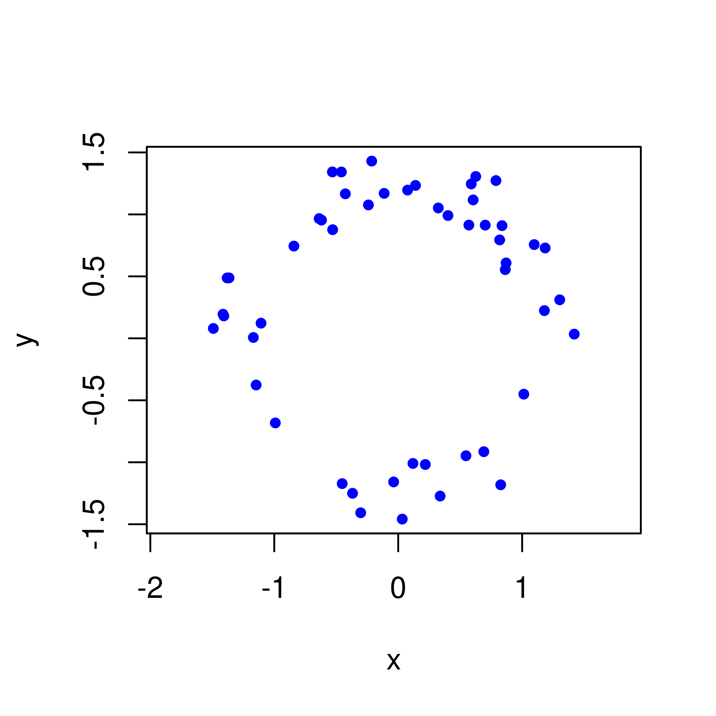

Now look at the persistence diagram:

PH.output <- alphaComplexDiag(X)
PD <- PH.output[["diagram"]]
plot(PD, asp=1, diagLim = c(0,1.5))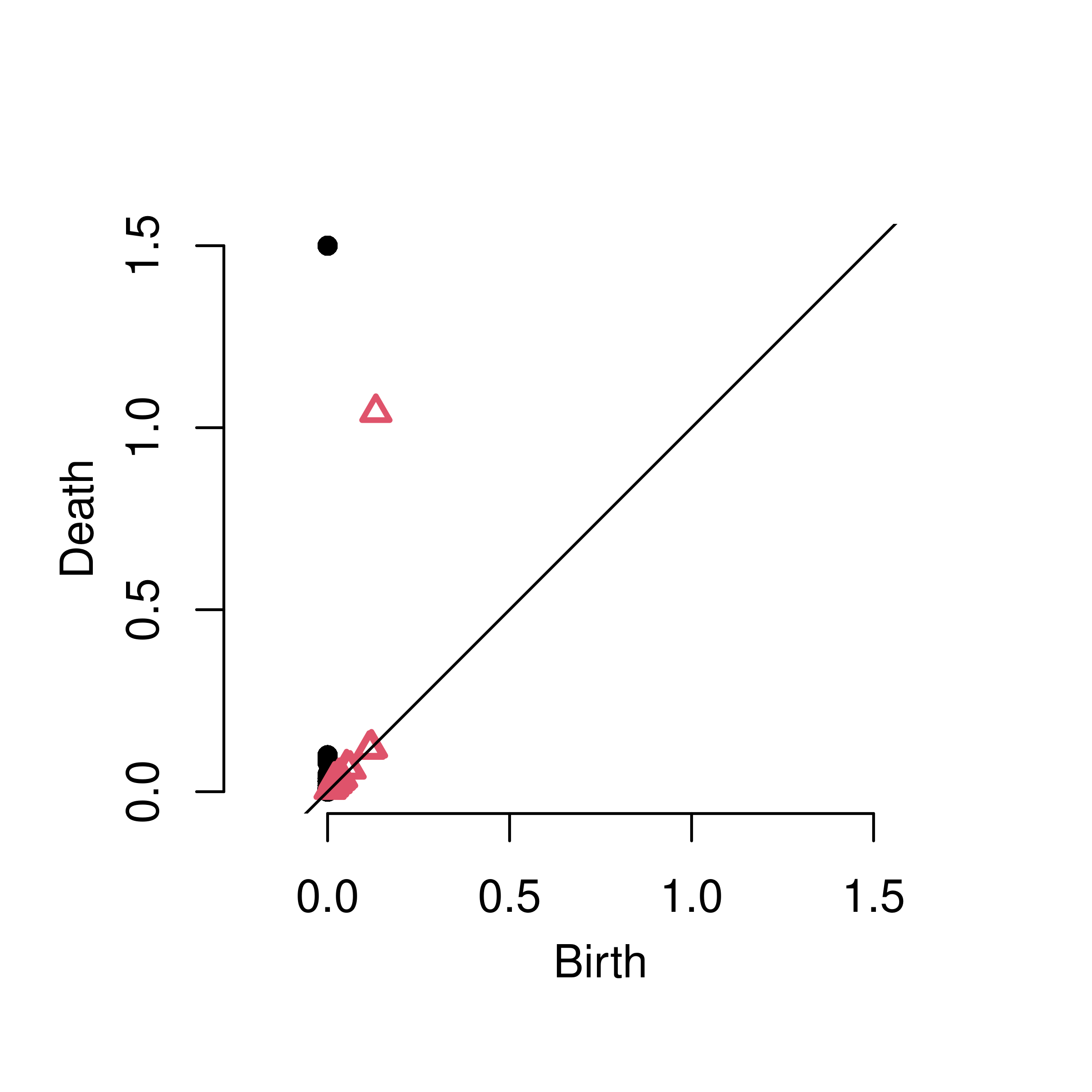

Here’s the barcode:

plot(PD, diagLim = c(0,1.5), barcode=TRUE)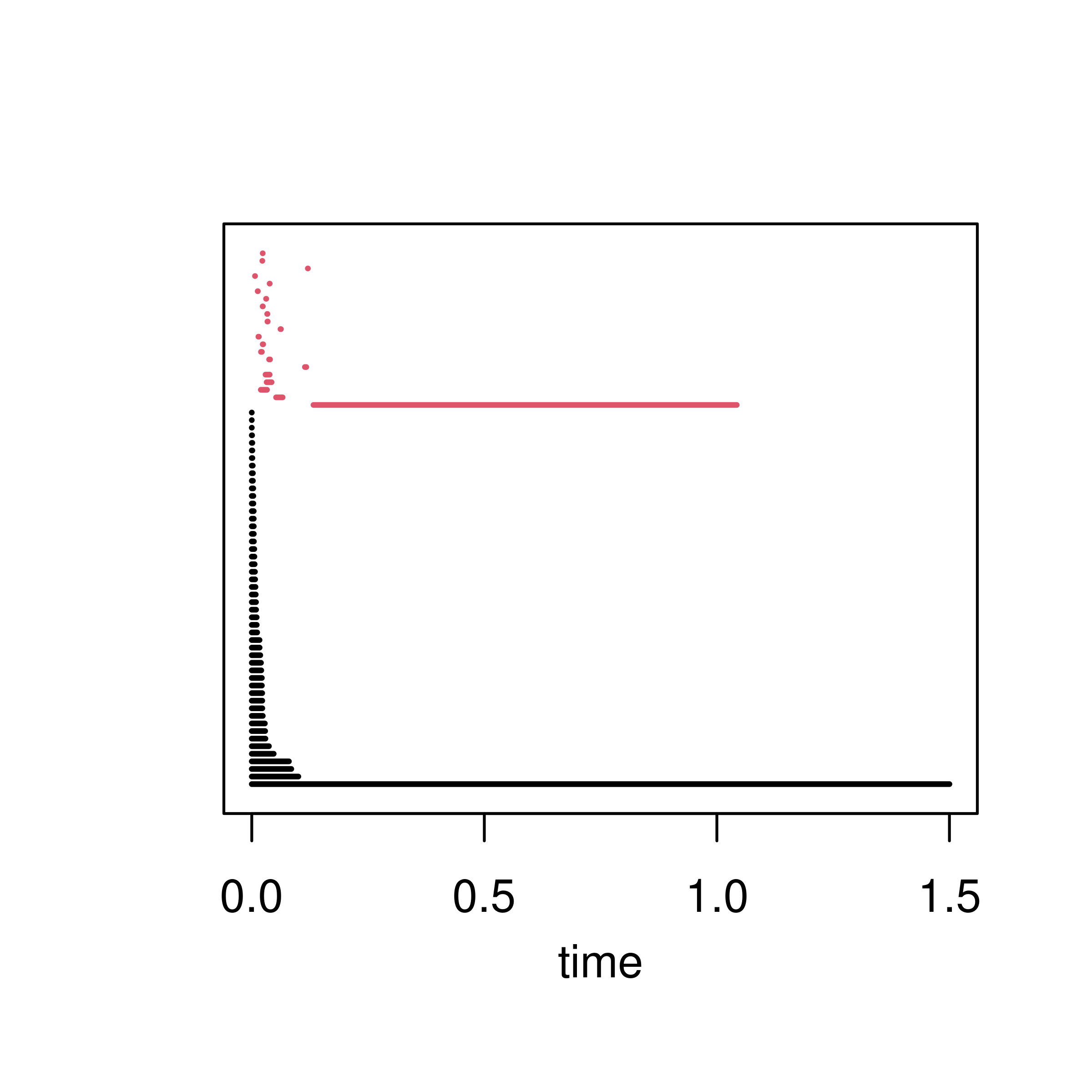

Here’s the landscape:

tseq <- seq(0, 1.5, 0.02)
plot(tseq, landscape(PD, dimension = 1, KK = 1, tseq), type = "l", xlab = "t", ylab = "landscape", asp = 1)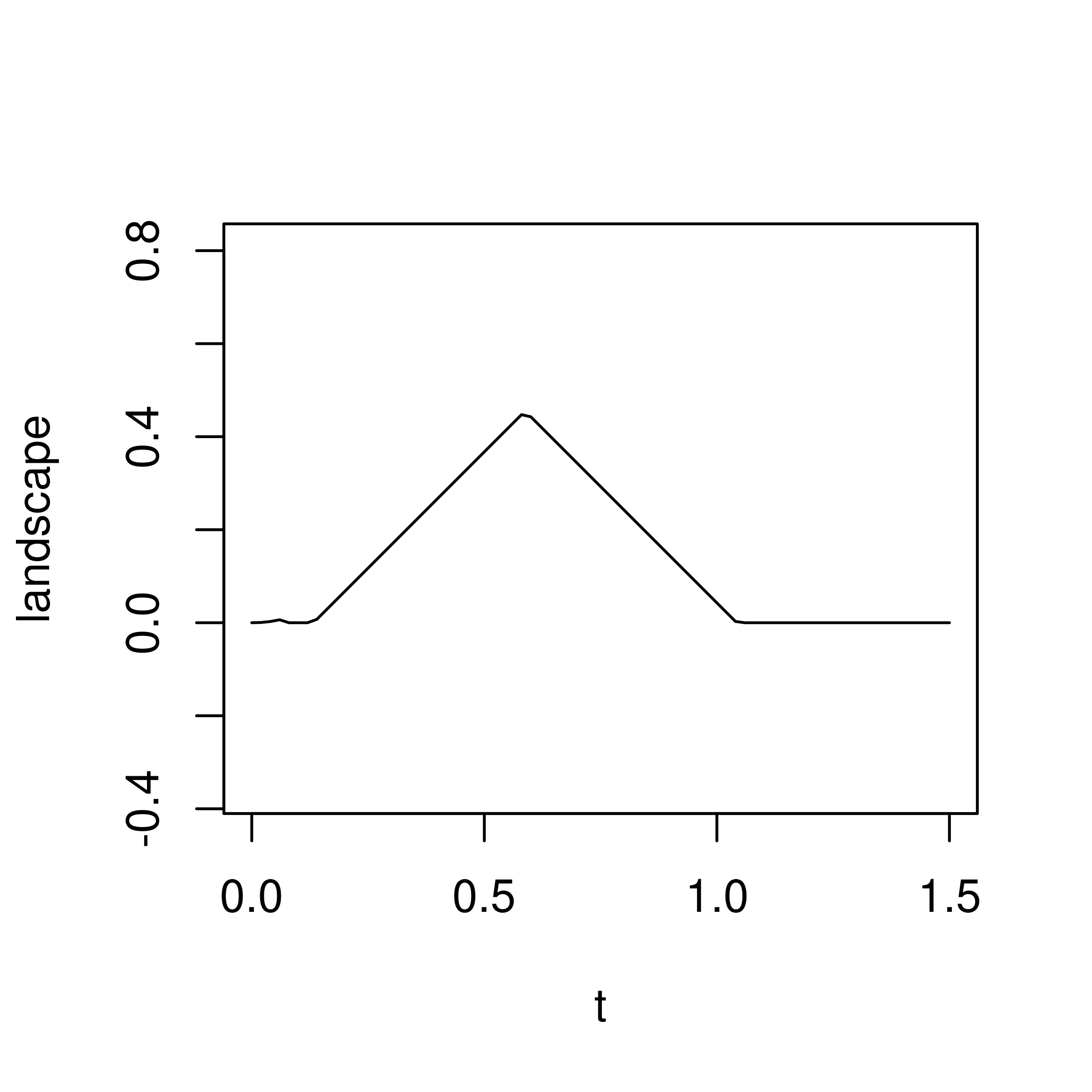

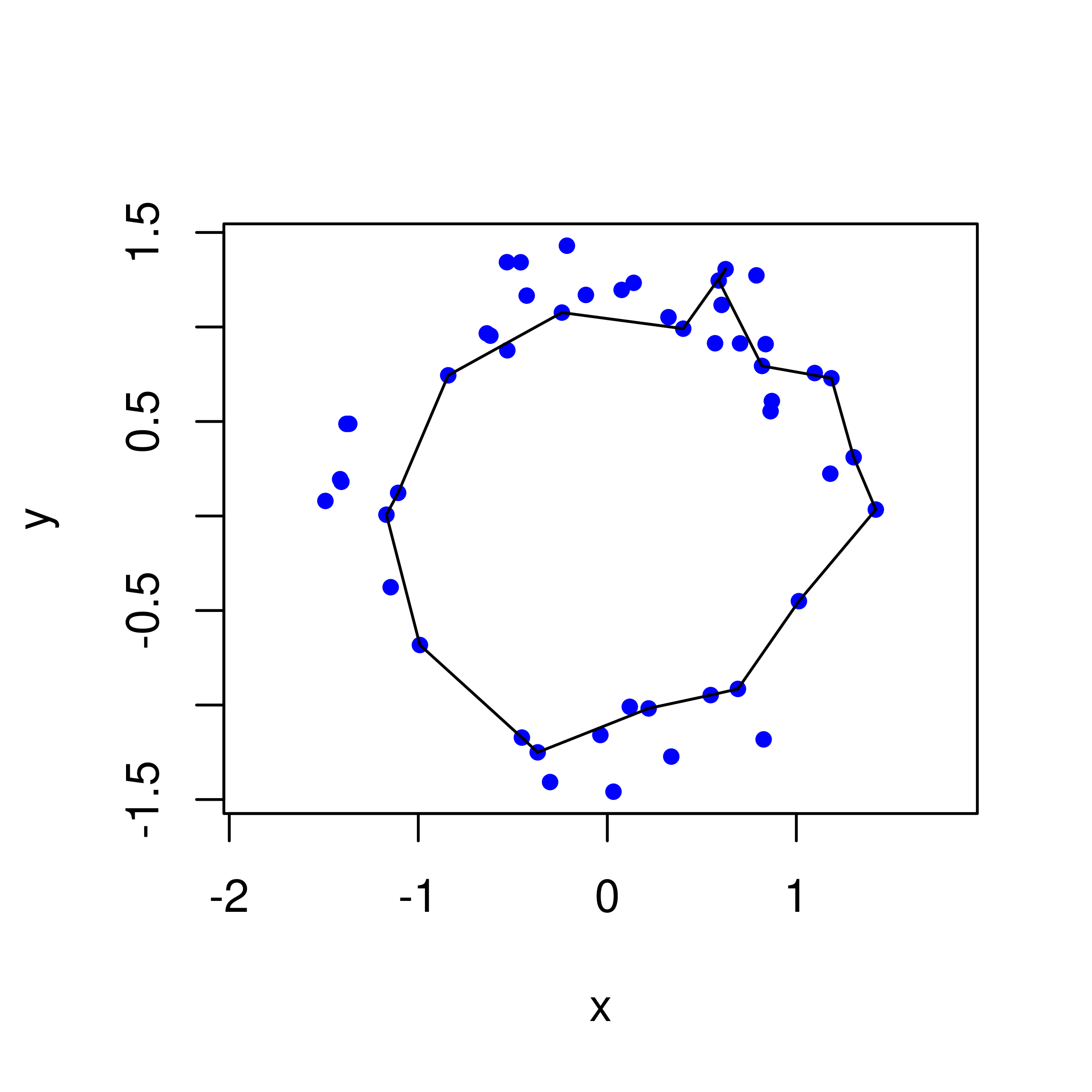
Now plot the longest persistent cycle.

PH.output <- ripsDiag(X, maxdimension = 1, maxscale = 2.2, library = c("GUDHI", "Dionysus"), location = TRUE)
PD <- PH.output[["diagram"]]
ones <- which(PD[, 1] == 1)
persistence <- PD[ones,3] - PD[ones,2]
cycles <- PH.output[["cycleLocation"]][ones[order(persistence, decreasing=TRUE)]]
plot(X, pch=20, col='blue', asp=1)
for (i in 1:dim(cycles[[1]])[1]){
    lines(cycles[[1]][i,,])
}