Neural networks are, essentially, stacked logistic regressions.

\[ x_1 = \text{logit}(W_1x+b_1) \qquad x_2 = \text{logit}(W_2x_1+b_2) \\ x_3 = \text{logit}(W_3x_2+b_3) \qquad x_4 = \text{logit}(W_4x_3+b_4) \]

Name comes from history.

Computational model of nervous systems:

Neurons are connected via synapses that connect axons to other neurons. Along the synapse, an electrical signal runs, causing the synapses to release chemical signals that in turn cause electrical signals in the next neuron.

Neurons tend to require sufficiently high build-up of incoming signals before they react, and may both be stimulated or inhibited by different incoming signals.

McCulloch-Pitts: 1943. Threshold logic.
Hebb: Late 1940s. unsupervised learning with neural plasticity.
Computational models of Hebbian learning emerged in the 1950s, leading to the perceptron (Rosenblatt 1958).

Neural networks got far more powerful once the biological view lost emphasis. Instead of neurons firing, neural networks can be understood as interleaved layers of

1. Linear transformations
2. Non-linear activation functions

Composed together these produce a function approximation system.

Common choices for the activation functions include sigmoids produced by \(\tanh\) or by logit, as well as softplus \(x\mapsto\log(1+\exp x)\) or ReLU \(x\mapsto\max(0,x)\).

A single layer perceptron has the shape \[ x \xrightarrow{Wx+b} \bullet \xrightarrow{f} \hat y \]

The single layer perceptron is essentially a linear classifier. For a logit activation, this is logistic regression.

Minsky and Papert (1969): single layer perceptrons cannot learn the XOR function

The perceptron can be extended to multiple layers by chaining several perceptrons on top of each other

\[ x \xrightarrow{W_1x+b_1} \bullet \xrightarrow{f} \bullet \xrightarrow{W_2x+b_2} \bullet \xrightarrow{f} \bullet \xrightarrow{W_3x+b_3} \bullet \xrightarrow{f} \hat y \]

1975 the backpropagation algorithm was developed, provided a method to train a multiple layer perceptron.

Backpropagation uses the chain rule of derivatives to flow prediction error \(E=L(y,\hat y)\) back through differentiable functions to calculate a global gradient \[ \nabla W = \left( \frac{\partial E}{\partial W_{ji}} ,\dots, \frac{\partial E}{\partial b_j},\dots \right) \]

With access to the gradient \(\nabla W\), we can use gradient descent methods to train the network.

Current best practices tend to use versions of Stochastic Gradient Descent: \[ W_{t+1} = W_t - \epsilon\nabla W + \delta \qquad \delta\sim\mathcal N(0,\sigma^2) \]

A lot of variations exist, decaying \(\epsilon\) and \(\sigma^2\), or replacing normal noise by a different noise model, …

Some time 2005-2010, neural networks started making a major come-back.

• GPU computation
• Access to large datasets
• New training approaches
• Decreased focus on AI in favor of machine learning tasks

The most commonly used layer type is the dense layer: \[ \hat y = f(Wx+b) \] with \(W\) a full matrix: every element in the vector \(x\) influences every element in \(\hat y\).

For very many network architecture, dense layers will show up as building blocks.

For image processing tasks, the position in an image of a single entry tends to not be an important aspect of the analysis. We would want to recognize the same thing wherever it occurs in an image.

CNNs provide a way to remove the spatial position dependency from the equation.

Images come into the system as 3-dimensional tensors, with shape \(w\times h\times c\) for \(w\) wide, \(h\) high images with \(c\) channels.

On these \(w\times h\times c\) observations, two new types of layers are introduced:

• Convolution layer: slide an \(x\times y\) window over the data, and use the same dense layer on each window to produce some output
• Pooling layer: slide an \(x\times y\) window over the data, and use some method to summarize the content in each window

Since they have VERY many degrees of freedom, neural network systems are prone to overfitting. This can be combated by

• Introducing regularization constraints: push the entries in the \(W_j\) to be small (in \(L_2\) or \(L_1\) norm)
• Introducing Dropout layers: layers that randomly remove parts of the information.

Having dropout layers forces the system to build redundancies – no information can be concentrated, otherwise it gets lost.

Logistic regression / logit perceptron

5 epochs: Training accuracy 63%, Accuracy 65%

Convolutions, Max-pooling and Dense/logistic regression endpoint

5 epochs: Training accuracy: 97%, Accuracy: 97%

One classical unsupervised use of neural networks is in autoencoders: to produce a dimensionality reduction, try to project data \(\mathbb R^p\to \mathbb R^d\) in such a way that a reconstruction \(\mathbb R^d\to\mathbb R^p\) is possible.

Use input data both as predictor and response. Read the activations in the narrow waist as the projection.

The narrowing part is called the encoder, the widening part the decoder.

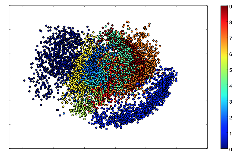
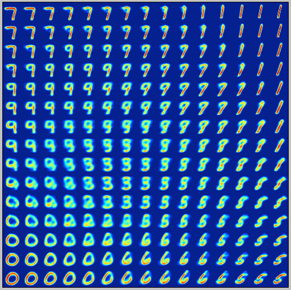
A variation of autoencoders produces a generative model with a probabilistic setup: learn parameters that describe a probability distribution on images.

The result is a sample-able "manifold" of things that look like tha data points.

https://blog.keras.io/building-autoencoders-in-keras.html

A recent and currently very popular unsupervised network type is the Generative Adversarial Network.

Basic idea: train two networks in tandem. One (the adversary) tries to distinguish artificial data from real data, the other one (the generator) tries to trick the adversary.

Keras is a Python library developed by Francois Chollet to make it easy and accessible to build neural networks.

((X,y), (Xt, yt)) = keras.datasets.mnist.load_data()
inp = Input(shape=(28,28))
x = Reshape((-1,))(inp)
outp = Dense(10, activation="softmax")(x)
model = Model(inputs=inp, outputs=outp)
model.compile(optimizer="rmsprop",
  loss="categorical_crossentropy",
  metrics=["accuracy"])
model.fit(X, to_categorical(y))
model.evaluate(Xt, to_categorical(yt))
model.predict(Xt)

inp = Input(shape=(28,28))
x = Reshape((28,28,1))(inp)
x = Conv2D(16, (3,3), activation="relu")(x)
x = MaxPool2D(2)(x)
x = Reshape((-1,))(x)
outp = Dense(10, activation="softmax")(x)
model = Model(inputs=inp, outputs=outp)

New feature. Includes features from Keras, but allows higher flexibility.

Eager execution skips the entire computation graph paradigm (see later) and instead executes all commands immediately.

Key entry point: write a model function

def model(features, labels, mode, params):
  ...

mode is an object with possible values ModeKeys.TRAIN, ModeKeys.EVAL and ModeKeys.PREDICT to distinguish different model uses.

Uniform estimation interface through instantiating an tf.estimator.Estimator

Also support for prewritten regression and classification: Linear and Dense Neural Network.

Computation graph.

1. Build a graph encoding the entire computation.
2. Start a computation session.
3. Feed data into compute graph.

Allows for extensive optimization and compute order management.

import tensorflow as tf

X_input = tf.placeholder(tf.float32, (None, 28, 28))
X_ = tf.reshape(X_input, (-1,28*28))

W = tf.get_variable("W", (28*28, 10))
b = tf.get_variable("b", 10)

logits = X_ @ W + b
out = tf.nn.softmax(logits)
y_out = tf.argmax(out, axis=1)

y_input = tf.placeholder(tf.int32, (None,))
y_reshaped = tf.one_hot(y_input, 10)

loss = tf.losses.softmax_cross_entropy(y_reshaped, logits)

optimizer = tf.train.AdamOptimizer()
train = optimizer.minimize(loss)

session = tf.Session()
session.run(tf.global_variables_initializer())

for epoch in range(250):
  _, loss_value = session.run((train, loss), 
                           {X_input: X, y_input: y})
  y_pred = session.run(y_out, {X_input: X})
  accuracy = sum(y_pred == y)/len(y)
  print(f"Epoch: {epoch}\tAccuracy: {accuracy:.4f}\tLoss: {loss_value:.4f}")

Keras and TensorFlow write log files to disk.

Separate application TensorBoard provides

Keras:

((X,y), (Xt, yt)) = keras.datasets.mnist.load_data()
inp = Input(shape=(28,28))
x = Reshape((-1,))(inp)
outp = Dense(10, activation="softmax")(x)
model = Model(inputs=inp, outputs=outp)
tb = keras.callbacks.TensorBoard(log_dir=f'./logs/{time.time()}', 
    histogram_freq=1, write_images=True, write_grads=True)
model.compile(optimizer="rmsprop",
  loss="categorical_crossentropy",
  metrics=["accuracy"])
model.fit(X, to_categorical(y), callbacks=[tb], epochs=10, 
  validation_split=0.1)
model.evaluate(Xt, to_categorical(yt))
model.predict(Xt)

Low-level TensorFlow

loss = tf.losses.softmax_cross_entropy(y_reshaped, logits)
tf.summary.scalar("loss", loss)

accuracy = tf.reduce_mean(tf.cast(y_out == y, tf.float32))
tf.summary.scalar("accuracy", accuracy)

merged = tf.summary.merge_all()
train_writer = tf.summary.FileWriter(
  f'./logs/{time.time()}', session.graph)

optimizer = tf.train.AdamOptimizer()
train = optimizer.minimize(loss)

session.run(tf.global_variables_initializer())

Low-level TensorFlow

for epoch in range(250):
  summary, _, acc = session.run(
    (merged, train, accuracy), 
    {X_input: X, y_input: y})
  train_writer.add_summary(summary)
  print(f"epoch: {epoch}\taccuracy: {accuracy}")